
Find research datasets worth reusing
Search datasets from major research repositories and use ShareScore to quickly assess how well each record supports discovery, access, and reuse.
1,487
datasets available to search
ShareScore release 0.9.0
Dataset results
1,487 results for “Tagging”
MulTI-Tag datasets and code
<p>This upload contain the code, .tsv fragment files, .rds files, and other interpreted files necessary to reproduce the single cell analysis presented the revised MulTI-Tag manuscript (https://doi.org/10.1101/2021.07.08.451691). Figure 2 includes datasets for K562, H1 hESC, and mixed K562-H1 co-profiled for H3K27me3 and H3K36me3; and K562, H1 hESC, and mixed K562-H1 co-profiled for multiple target combinations in the same experiment (H3K27me3-PolIIS5P, H3K27me3-H3K9me3, H3K27me3-H3K4me1, H3K27me3-H3K36me3). Figure 3 includes datasets for K562 and H1 co-profiled for H3K27me3, H3K4me2, and H3K36me3. Figure 4 includes datasets for H1 hESCs differentiated to three germ layers (Ectoderm, Endoderm, and Mesoderm), with timepoints collected every 24 hours, and co-profiled for H3K27me3, H3K4me1, and H3K36me3.</p>
American Beaver: GPS and VHF tag data from resident and translocated beavers on the Price and San Rafael Rivers, Utah
<p>Wildlife translocations can dramatically alter animal movement behavior. Thus, identifying common movement patterns post-translocation can aid in setting expectations and anticipating animal behavior in subsequent efforts. American and Eurasian beavers (Castor canadensis; C. fiber) are frequently translocated for reintroduction efforts, to mitigate human-wildlife conflict, and for use as an ecosystem restoration tool. However, little is known about movement behavior of translocated beavers post-release, especially in desert rivers where resources are patchy and dynamic. We identified space-use patterns to develop an expectation framework of beaver movement behavior for future beaver-assisted restoration efforts. We captured, tagged, translocated, and monitored 41 nuisance American beavers in desert river restoration sites on the Price and San Rafael Rivers, Utah, USA, and compared their space use to 16 resident beavers. We tracked beavers 2-7 times per week from May through October in 2019 and 2020 via GPS locations and radio-telemetry, and from May 2019 through March 2021 via passive integrated antennae installed in the rivers. Resident adult beavers were detected at a mean maximum distance of 0.86 ± 0.21 river kilometers (km; ±1 SE), while resident subadult (11.00 ± 4.24 km), translocated adult (19.69 ± 3.76 km), and translocated subadult (21.09 ± 5.54 km) beavers were detected at substantially greater maximum distances. Based on coarse-scale movement models, translocated and resident subadult beavers moved substantially farther from release sites and faster than resident adult beavers up to six months post-release. In contrast, based on fine-scale, short-term movement models over 5-minute intervals, we observed similar median distance traveled between resident adult and translocated beavers. Our findings suggest day-to-day activities such as foraging and resting were largely unaltered by translocation, but translocated beavers exhibited coarse-scale movement behavior most similar to dispersal by resident subadults. Coarse-scale movement rates decreased with time since release, suggesting that translocated beavers adjusted to the novel environment over time and eventually settled into a home range similar to resident adult beavers. This is the first study comparing resident and translocated beaver movement behavior in the same system. Understanding translocated beaver movement behavior in response to a novel desert system can help future beaver-assisted restoration efforts to identify appropriate release sites and strategies.</p>
Data from: A shared numerical magnitude representation evidenced by the distance effect in frequency-tagging EEG
<p>Humans can effortlessly abstract numerical information from various codes and contexts. However, whether the access to the underlying magnitude information relies on common or distinct brain representations remains highly debated. Here, we recorded electrophysiological responses to periodic variation of numerosity (every five items) occurring in rapid streams of numbers presented at 6Hz in randomly varying codes – Arabic digits, number words, canonical dot patterns and finger configurations. Results demonstrated that numerical information was abstracted and generalized over the different representation codes by revealing clear discrimination responses (at 1.2 Hz) of the deviant numerosity from the base numerosity, recorded over parieto-occipital electrodes. Crucially, and supporting the claim that discrimination responses reflected magnitude processing, the presentation of a deviant numerosity distant from the base (e.g., base "2" and deviant "8") elicited larger right-hemispheric responses than the presentation of a close deviant numerosity (e.g., base "2" and deviant "3"). This finding nicely represents the neural signature of the distance effect, an interpretation further reinforced by the clear correlation with individuals' behavioral performance in an independent numerical comparison task. Our results, therefore, provide for the first time unambiguously a reliable and specific neural marker of a magnitude representation that is shared among several numerical codes.</p>
Semantically tagged Finnish Wikipedia 2017
<p><strong>Description of FI Wikipedia 2017 tagging</strong></p> <p><strong>Kimmo Kettunen</strong></p> <p><strong>University of Eastern Finl</strong><strong>and</strong></p> <p>The tagged data contains the texts of the Finnish Wikipedia of 2017. It has been first tagged syntactically in the Language Bank of Finland using the available UD2 tagger version of the Mylly service (https://mylly.rahtiapp.fi/home).</p> <p>Semantic tags to the UD2 parse have been added using a lexical semantic tagger FiST (Kettunen, 2019, <a href="https://aclanthology.org/W19-0306/">https://aclanthology.org/W19-0306/</a>).</p> <p>This published version has been condensed to a format where each analysed word contains the</p> <p>1. original running word form,</p> <p>2. lemma of the word form from UD2 parse,</p> <p>3. part-of-speech of the word from FiST</p> <p>4. semantic tag(s) for the word from FiST, and</p> <p>5. syntactic function of the word from UD2 parse.</p> <p>Semantic tags used are explained in this UCREL Semantic Analysis System (USAS) document: <a href="https://ucrel.lancs.ac.uk/usas/USASSemanticTagset.pdf">https://ucrel.lancs.ac.uk/usas/USASSemanticTagset.pdf</a></p> <p>Tagging includes all the semantic tags available for the word, as FiST does not perform disambiguation. Unknown words for the tagger are marked with tag Z99. Punctuation is tagged with PUNCT and numbers with NUMB. Lines beginning with # are output of UD2 and contain document, paragraph and sentence information.</p> <p>The output contains 6 415 027 sentences and 98.81 million lines. Lexical coverage of the semantic tagging is 76.59 %</p> <p><strong>Examples of output</strong></p> <p># newdoc</p> <p># newpar</p> <p># sent_id = 1</p> <p># text = Amsterdam</p> <p>Amsterdam#Amsterdam#Proper#Z2 root</p> <p># newpar</p> <p># sent_id = 2</p> <p># text = Amsterdam on Alankomaiden pääkaupunki.</p> <p>Amsterdam#Amsterdam#Proper#Z2 nsubj:cop</p> <p>on#olla#Verb#A3+ A1.1.1 M6 Z5 cop</p> <p>Alankomaiden#Alankomaat#Proper#Z2 nmod:poss</p> <p>pääkaupunki#pääkaupunki#Noun#M7 root</p> <p>. PUNCT</p>
Tag urbain Le Gabut, La Rochelle
14 Photographies. Modélisation 3D A. Laurent 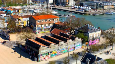 Source: Objaverse 1.0 / Sketchfab
Public tags added to resources in Trove, 2008 to 2024
<p>This dataset contains details of 2,495,958 unique public tags added to 10,403,650 resources in <a href="https://trove.nla.gov.au/">Trove</a> between August 2008 and June 2024. I harvested the data using the Trove API and saved it as a CSV file with the following columns:</p> <ul> <li>`tag` – lower-cased text tag</li> <li>`date` – date the tag was added</li> <li>`zone` – API zone containing the tagged resource</li> <li>`record_id` – the identifier of the tagged resource</li> </ul> <p>I've documented the method used to harvest the tags in <a href="https://github.com/GLAM-Workbench/trove-lists/blob/master/harvest-tags.ipynb">this notebook</a>.</p> <p>Using the `zone` and `record_id` you can find more information about a tagged item. To create urls to the resources in Trove:</p> <ul> <li>for resources in the 'book', 'article', 'picture', 'music', 'map', and 'collection' zones add the `record_id` to `https://trove.nla.gov.au/work/`</li> <li>for resources in the 'newspaper' and 'gazette' zones add the `record_id` to `https://trove.nla.gov.au/article/`</li> <li>for resources in the 'list' zone add the `record_id` to `https://trove.nla.gov.au/list/`</li> </ul> <p>Notes:</p> <ul> <li>Works (such as books) in Trove can have tags attached at either work or version level. This dataset aggregates all tags at the work level, removing any duplicates.</li> <li>A single resource in Trove can appear in multiple zones – for example, a book that includes maps and illustrations might appear in the 'book', 'picture', and 'map' zones. This means that some of the tags will essentially be duplicates – harvested from different zones, but relating to the same resource. Depending on your needs, you might want to remove these duplicates.</li> <li>While most of the tags were added by Trove users, more than 500,000 tags were added by Trove itself in November 2009. I think these tags were automatically generated from related Wikipedia pages. Depending on your needs, you might want to exclude these by limiting the date range or zones.</li> <li>User content added to Trove, including tags, is available for reuse under a CC-BY-NC licence.</li> </ul> <p>See <a href="https://github.com/GLAM-Workbench/trove-lists/blob/master/analyse_tags.ipynb">this notebook</a> for some examples of how you can manipulate, analyse, and visualise the tag data.</p>
Figure 1 in Quantitative phosphoproteomic analysis of chicken DF-1 cells infected with Eimeria tenella, using tandem mass tag (TMT) and parallel reaction monitoring (PRM) mass spectrometry
Figure 1. Proportion of serine, threonine, and tyrosine in phosphorylation sites.
The burden of research: Effects of GPS tags on metabolic physiology of a small passerine
<p>Statistical code & corresponding datasets for "The burden of research: Effects of GPS tags on metabolic physiology of a small passerine" submitted to <em>Ornithilogical Applications.</em></p>
Huntingtin Exon 1 Q16 and Q46 pET32a thioredoxin tagged expression and purification 2018/04/09
<p>Huntingtin structure-function open lab notebook project. Huntingtin Exon 1 Q16 and Q46 pET32a thioredoxin tagged expression and purification 2018/04/09.</p>
Huntingtin Exon 1 Q16 and Q46 pET32a thioredoxin tagged expression and purification 2018/04/02
<p>Huntingtin structure-function open lab notebook project. Huntingtin Exon 1 Q16 and Q46 pET32a thioredoxin tagged, attempted expression and purification 2018/04/02</p>
A New Annotation Scheme for the Sejong Part-of-speech Tagged Corpus
<p>We produce Sejong-style morphological analysis and part-of-speech tagging results which have been the de facto standard for Korean language processing by using UDPipe (http://ufal.mff.cuni.cz/udpipe) </p> <p> </p> <p>udpipe --tokenize --tag sjmorph.model input > output</p> <p>see https://github.com/jungyeul/sjmorph</p>
BPASS pair-instability supernova tagging
<p>These data contain the tagging of individual models from the BPASS population for different pair-instability supernova prescriptions. The data is stored as a pandas DataFrame with the identifier: `rates`.</p> <pre><code>df = pd.read_hdf(f'22_3_2024_{MET}.h5', 'rates')</code></pre> <p>The following data columns are available:</p> <ul> <li>filenames: the BPASS model name. Note: some merger models in the v2.2 release failed before reaching/avoiding the PISN regime. These have been rerun and often do not lead to a PISN.</li> <li>model_imf: the weight of the model; directly from BPASS</li> <li>types: the type of model (merger, primary, secondary, single, effectively single)</li> <li>mixed_imf: the weight of the model for secondaries; directly from BPASS</li> <li>mixed_age: the start age of a secondary model due to rejuvenation; directly from BPASS</li> <li>total_mass: the total mass of the PISN progenitor model at the end of the model</li> <li>helium_mass: the total helium core mass of the PISN progenitor model at the end of the model</li> <li>co_mass: the total carbon-oxygen core mass of the PISN progenitor model at the end of the model</li> </ul> <p>The remaining columns are "booleans" for the different PISN prescriptions:</p> <ul> <li>standard: The fiducial model used in Briel et al. (2023)</li> <li>old_bpass: The original BPASS tagging used in Briel et al. (2022)</li> <li>CO_only: Tagging with only the CO core >= 60 Msun as a limit</li> <li>merchant: PISN limits from Marchant et al. (2019)</li> <li>noH: standard tagging but no hydrogen present.</li> <li> ['0', '1', '2', '3', '4', '5']: different formation channels, shifted one up from the BPASS model identification</li> <li>['R150', 'R175', 'R200', 'R225', 'R250', 'He70', 'He80', 'He90', 'He100', 'He110', 'He120', 'He130']: tagging based on each light curve.</li> </ul> <p>This can be used to get the metallicity bias functions (number of events per Msun over metallicity) or to create new taggings.</p> <p>For example, below we use both the existing tagging with `model_imf` weights to get the rate of PISN at each metallicity and we create a new tagging `shifted_up`, which is a tagging where the PISN limit is shifted upwards.</p> <p> </p> <pre><code>import pandas as pd import numpy as np from hoki.constants import BPASS_METALLICITIES # from Kaasen et al. 2008 paper envelopes = np.array([70.9, 79.4, 84.4, 96.8, 112.3, 0, 0, 0, 0, 0, 0, 0]) helium_cores = np.array([72.0, 84.4, 96.7, 103.5, 124.0, 70, 80, 90, 100, 110, 120, 130]) curve_models = [ 'R150', 'R175', 'R200', 'R225', 'R250', 'He70', 'He80', 'He90', 'He100', 'He110', 'He120', 'He130'] bias_functions = pd.DataFrame({'standard':np.zeros(13), 'standard_old':np.zeros(13), 'CO_only':np.zeros(13), 'marchant':np.zeros(13), 'shift_up':np.zeros(13), 'old_BPASS':np.zeros(13), 'He_only':np.zeros(13), 'primary':np.zeros(13), 'secondary':np.zeros(13), 'QHE':np.zeros(13), 'merger':np.zeros(13), 'single':np.zeros(13), 'R150':np.zeros(13), 'R175':np.zeros(13), 'R200':np.zeros(13), 'R225':np.zeros(13), 'R250':np.zeros(13), 'He70':np.zeros(13), 'He80':np.zeros(13), 'He90':np.zeros(13), 'He100':np.zeros(13), 'He110':np.zeros(13), 'He120':np.zeros(13), 'He130':np.zeros(13)}) bias_functions.index = BPASS_METALLICITIES for MET in BPASS_METALLICITIES[:-4]: print(MET) df = pd.read_hdf(f'PISN_data_{MET}.h5', 'rates') for i in curve_models: mask = (df['co_mass'] >=60) & (df['helium_mass'] < 133) & (df[i] == 1) bias_functions.loc[MET, i] = np.sum(df[mask]['model_imf'])/1e6 mask = (df['co_mass'] >=60) & (df['helium_mass'] < 133) bias_functions.loc[MET, 'standard'] = np.sum(df[mask]['model_imf'])/1e6 bias_functions.loc[MET, 'standard_old'] = np.sum(df[df['standard'] == 1]['model_imf'])/1e6 mask = (df['helium_mass'] >=64) & (df['helium_mass'] < 133) bias_functions.loc[MET, 'old_BPASS'] = np.sum(df[mask]['model_imf'][mask])/1e6 mask = (df['co_mass'] >= 60) bias_functions.loc[MET, 'CO_only'] = np.sum(df[df['CO_only'] == 1]['model_imf'][mask])/1e6 mask = (df['helium_mass'] >=60.8) & (df['helium_mass'] < 124) bias_functions.loc[MET, 'marchant'] = np.sum(df[df['marchant'] == 1]['model_imf'][mask])/1e6 bias_functions.loc[MET, 'noH'] = np.sum(df[df['noH'] == 1]['model_imf'])/1e6 mask = (df['helium_mass'] >=90) & (df['helium_mass'] < 180) bias_functions.loc[MET, 'shift_up'] = np.sum(df[mask]['model_imf'])/1e6 mask = np.isclose(df['total_mass'] - df['helium_mass'], 0, atol=0.1) & (df['helium_mass'] < 133) & (df['co_mass'] >=60) bias_functions.loc[MET, 'He_only'] = np.sum(df[mask]['model_imf'])/1e6 mask = (df['co_mass'] >=60) & (df['helium_mass'] < 133) bias_functions.loc[MET, 'merger'] = np.sum(df[(df['types'] == 0) & mask]['model_imf'])/1e6 bias_functions.loc[MET, 'single'] = np.sum(df[((df['types'] == -1) | (df['types'] == 3)) & mask]['model_imf'])/1e6 bias_functions.loc[MET, 'primary'] = np.sum(df[(df['types'] == 1) & mask]['model_imf'])/1e6 bias_functions.loc[MET, 'secondary'] = np.sum(df[(df['types'] == 2) & mask]['model_imf'])/1e6 bias_functions.loc[MET, 'QHE'] = np.sum(df[(df['types'] == 4) & mask]['model_imf'])/1e6</code></pre>
Figure 2 in Variability in Reception Duration of Dual Satellite Tags on Sea Turtles Tracked in the Pacific Ocean
Figure 2. Example of dual tag attachment to a loggerhead turtle.
FIGURE 3 in Radiotagging a long-distance migratory characid fish: reproduction after surgery, tag losses, and effects in weight
FIGURE 3 | Fecundity (oocytes by gram of body weight) compared among treatments.
Fig. 2 in Effect of anesthetic, tag size, and surgeon experience on postsurgical recovering after implantation of electronic tags in a neotropical fish: Prochilodus lineatus (Valenciennes, 1837) (Characiformes: Prochilodontidae)
Fig. 2. Examples of tag expulsion (left) and antenna migration (right) of Prochilodus lineatus.
Fig. 3 in Effect of anesthetic, tag size, and surgeon experience on postsurgical recovering after implantation of electronic tags in a neotropical fish: Prochilodus lineatus (Valenciennes, 1837) (Characiformes: Prochilodontidae)
Fig. 3. Healthy (left) and infected (right) viscera on necropsy of Prochilodus lineatus.
Fig. 1 in Effect of anesthetic, tag size, and surgeon experience on postsurgical recovering after implantation of electronic tags in a neotropical fish: Prochilodus lineatus (Valenciennes, 1837) (Characiformes: Prochilodontidae)
Fig. 1. Criteria and examples for the surgical and postsurgical rankings.
Nanotate - Tag distribution
<p>232 parts-of-speech from open access experimental protocols in biology were tagged by using the Nanotate tool with the six available categories (sample, equipment, reagent, input, output, step).</p>
The analysis of composition and abundance of the raft proteome of microglia using a tandem mass tag (TMT)-based quantitative proteomic analysis.
<p>To determine the proteins in the membrane raft, we used the TMT-labeling and nano-liquid chromatography mass spectrometry (nano-LC-MS/MS) analysis by Creative Proteomics (NY, USA; https://www.creative-proteomics.com/). Rat primary microglia were treated with IL-6 (25 ng/ml) for 15 min. Membrane rafts were obtained by flotation assay. Samples were prepared from three independent experiments. Proteins in equal volumes of raft fractions were digested with trypsin, desalted, and labeled with a TMT reagent (Thermo Fisher Science). The TMT-labeled peptides were fractionated and analyzed by nano-LC-MS/MS. The resulting MS/MS data were analyzed and searched against the rat protein database using Proteome Discoverer 2.1.</p>
scCUT&Tag-pro datasets
<p>The datasets uploaded here were generated using scCUT&Tag-pro for six single-cell histone modification marks: H3K4me1, H3K4me2, H3K4me3, H3K27ac, H3K27me3, H3K9me3. </p> <p>Please note that the following commands can be used to update the Fragment file in each object. The commands below should be used in place of the commands listed in README.txt</p> <pre>Fragments(obj) <- NULL Fragments(obj) <- CreateFragmentObject(path = file.path, cells = Cells(obj))</pre>
ScienceDex guides
Understand access before you commit
These curated guides explain access requirements, typical timelines, costs, and reuse considerations for widely used research datasets.
Allen Brain Atlas
Allen Brain Atlas is an Allen Institute collection of brain map atlases, datasets, APIs, and analysis tools covering mouse, human, and non-human primate brain resources.
Annotated Behaviour and Observability Dataset (ABODe)
ABODe is a University of Edinburgh DataShare dataset for behavior classification in group-housed mice using home-cage video, identities, bounding boxes, ground-plate positions, and annotator labels.
DANDI Archive for NWB datasets
DANDI is a BRAIN Initiative archive for publishing and sharing neurophysiology data, including electrophysiology, optophysiology, and behavioral data packaged as NWB and related standards.
International Brain Laboratory public data
The International Brain Laboratory public data releases expose standardized mouse decision-making experiments, including Neuropixels recordings, widefield calcium imaging, behavior, and session metadata accessed through the ONE API.
OpenNeuro
OpenNeuro is a free, open platform for sharing neuroimaging datasets, with public search, dataset pages, and download paths for web, S3, DataLad, and the OpenNeuro CLI.