
Find research datasets worth reusing
Search datasets from major research repositories and use ShareScore to quickly assess how well each record supports discovery, access, and reuse.
853
datasets available to search
ShareScore release 0.9.0
Dataset results
853 results for “sign”
Visitor Sign at Tainaron
<p>Tourist sign greeting the visitor to the "Sanctuary and Death Oracle of Poseidon Tainarios" in English and Greek. Tainaron, Mani Peninsula, Lakonia, Greece.</p>
Chinese Chemical Safety Signs (CCSS)
<p><strong>Chinese Chemical Safety Signs (CCSS)</strong></p> <p>This dataset is compiled as a benchmark for recognizing chemical safety signs from images. We provide both the dataset and the experimental results.</p> <p><strong><em>1. The Dataset</em></strong></p> <p>The complete dataset is contained in the folder <code>ccss/data</code>. The images include signs based on the Chinese standard "Safety Signs and their Application Guidelines" (GB 2894-2008) for safety signs in chemical environments. This standard, in turn, refers to the standards ISO 7010 (Graphical symbols – Safety Colours and Safety Signs – Safety signs used in workplaces and public areas), GB/T 10001 (Public Information Graphic Symbols for Signs), and GB 13495 (Fire Safety Signs)</p> <p><strong>1.1. Image Collection</strong></p> <p>We collect photos of commonly used chemical safety signs in chemical laboratories and chemistry teaching. For a discussion of the standards we base our collections, refer to the book "Talking about Hazardous Chemicals and Safety Signs" for common signs, and refer to the safety signs guidelines (GB 2894-2008).</p> <ul> <li>The shooting was mainly carried out in 6 locations, namely on the road, in a parking lot, construction walls, in a chemical laboratory, outside near big machines, and inside the factory and corridor.</li> <li>Shooting scale: Images in which the signs appear in small, medium and large scales were taken for each location by shooting photos from different distances.</li> <li>Shooting light: good lighting conditions and poor lighting conditions were investigated.</li> <li>Part of the images contain multiple targets and the other part contains only single signs.</li> </ul> <p>Under all conditions, a total of 4650 photos were taken in the original data. These were expanded to 27,900 photos were via data enhancement. All images are located in folder <code>ccss/data/JPEGImages</code>.</p> <p>The file <code>ccss/data/features/enhanced_data_to_original_data.csv</code> provides a mapping between the enhanced image name and the corresponding original image.</p> <p><strong>1.2. Annotation and Labelimg</strong></p> <p>We use Labelimg as labeling tool, which, in turn, uses the PASCAL-VOC labelimg format. The annotation is stored in the folder <code>ccss/data/Annotations</code>.</p> <p>Faster R-CNN and SSD are two algorithms that use this format. When training YOLOv5, you can run <code>trans_voc2yolo.py</code> to convert the XML file in PASCAL-VOC format to a txt file.</p> <p>We provide further meta-information about the dataset in form of a CSV file <code>features.csv</code> which notes, for each image, which other features it has (lighting conditions, scale, multiplicity, etc.). We apply the COCO standard for deciding whether a target is small, medium, or large in size.</p> <p><strong>1.3. Dataset Features</strong></p> <p>As stated above, the images have been shot under different conditions. We provide all the feature information in folder <code>ccss/data/features</code>. For each feature, there is a separate list of file names in that folder. The file <code>ccss/data/features/features_on_original_data.csv</code> is a CSV file which notes all the features of each original image.</p> <p><strong>1.4. Dataset Division</strong></p> <p>The data set is fixedly divided into 7:3 training set and test set. You can find the corresponding image names in the files <code>ccss/data/training_data_file_names.txt</code> and <code>ccss/data/test_data_file_names.txt</code>.</p> <p><strong><em>2. Baseline Experiments</em></strong></p> <p>We provide baseline results with five models, namely Faster R-CNN (R), Faster R-CNN (M), SSD, YOLOv3-spp, and YOLOv5. All code and results is given in folder <code>ccss/experiment</code>.</p> <p><strong>2.2. Environment and Configuration:</strong></p> <ul> <li>Single Intel Core i7-8700 CPU</li> <li>NVIDIA GTX1060 GPU</li> <li>16 GB of RAM</li> <li>Python: 3.8.10</li> <li>pytorch: 1.9.0</li> <li>pycocotools: pycocotools-win</li> <li>Visual Studio 2017</li> <li>Windows 10</li> </ul> <p><strong>2.3. Applied Models</strong></p> <p>The source codes and results of the applied models is given in folder <code>ccss/experiment</code> with sub-folders corresponding to the model names.</p> <p><em>2.3.1. Faster R-CNN</em></p> <ul> <li>Faster R-CNN (R) has the backbone resnet50+fpn. <ul> <li>we downloaded the pre-training weights from <a href="https://download.pytorch.org/models/fasterrcnn_resnet50_fpn_coco-258fb6c6.pth">https://download.pytorch.org/models/fasterrcnn_resnet50_fpn_coco-258fb6c6.pth</a></li> <li>we modify the type information of the JSON file to match our application.</li> <li>run <code>train_res50_fpn.py</code></li> <li>finally, the weights trained by the training set.</li> </ul> The Faster R-CNN (R) source code used in our experiment is given in folder <code>ccss/experiment/sources/faster_rcnn (R)</code>. The weights of the fully-trained Faster R-CNN (R) model are stored in file <code>ccss/experiment/trained_models/faster_rcnn (R).pth</code>. The performance measurements of Faster R-CNN (R) are stored in folder <code>ccss/experiment/performance_indicators/faster_rcnn (R)</code>.</li> <li>Faster R-CNN (M) has the backbone mobilenetv2. <ul> <li>backbone: MobileNetV2.</li> <li>we modify the type information of the JSON file to match our application.</li> <li>run <code>train_mobilenetv2.py</code></li> <li>finally, the weights trained by the training set.</li> </ul> The Faster R-CNN (M) source code used in our experiment is given in folder <code>ccss/experiment/sources/faster_rcnn (M)</code>. The weights of the fully-trained Faster R-CNN (M) model are stored in file <code>ccss/experiment/trained_models/faster_rcnn (M).pth</code>. The performance measurements of Faster R-CNN (M) are stored in folder <code>ccss/experiment/performance_indicators/faster_rcnn (M)</code>.</li> </ul> <p><em>2.3.2. SSD</em></p> <ul> <li>backbone: resnet50</li> <li>we downloaded pre-training weights from <a href="https://download.pytorch.org/models/resnet50-19c8e357.pth">https://download.pytorch.org/models/resnet50-19c8e357.pth</a></li> <li>the same training method as Faster R-CNN is applied.</li> </ul> <p>The SSD source code used in our experiment is given in folder <code>ccss/experiment/sources/ssd</code>. The weights of the fully-trained SSD model are stored in file <code>ccss/experiment/trained_models/ssd.pth</code>. The performance measurements of SSD are stored in folder <code>ccss/experiment/performance_indicators/ssd</code>.</p> <p><em>2.3.3. YOLOv3-spp</em></p> <ul> <li>backbone: DarkNet53</li> <li>we modified the type information of the XML file to match our application</li> <li>run <code>trans_voc2yolo.py</code> to convert the XML file in VOC format to a txt file.</li> <li>the weights used are: yolov3-spp-ultralytics-608.pt.</li> </ul> <p>The YOLOv3-spp source code used in our experiment is given in folder <code>ccss/experiment/sources/yolov3-spp</code>. The weights of the fully-trained YOLOv3-spp model are stored in file <code>ccss/experiment/trained_models/yolov3-spp.pt</code>. The performance measurements of YOLOv3-spp are stored in folder <code>ccss/experiment/performance_indicators/yolov3-spp</code>.</p> <p><em>2.3.4. YOLOv5</em></p> <ul> <li>backbone: CSP_DarkNet</li> <li>we modified the type information of the XML file to match our application</li> <li>run <code>trans_voc2yolo.py</code> to convert the XML file in VOC format to a txt file.</li> <li>the weights used are: yolov5s.</li> </ul> <p>The YOLOv5 source code used in our experiment is given in folder <code>ccss/experiment/sources/yolov5</code>. The weights of the fully-trained YOLOv5 model are stored in file <code>ccss/experiment/trained_models/yolov5.pt</code>. The performance measurements of YOLOv5 are stored in folder <code>ccss/experiment/performance_indicators/yolov5</code>.</p> <p><strong>2.4. Evaluation</strong></p> <p>The computed evaluation metrics as well as the code needed to compute them from our dataset are provided in the folder <code>ccss/experiment/performance_indicators</code>. They are provided over the complete test st as well as separately for the image features (over the test set).</p> <p><strong><em>3. Code Sources</em></strong></p> <ol> <li>Faster R-CNN (R and M) <ul> <li><a href="https://github.com/WZMIAOMIAO/deep-learning-for-image-processing/tree/master/pytorch_object_detection/faster_rcnn">https://github.com/WZMIAOMIAO/deep-learning-for-image-processing/tree/master/pytorch_object_detection/faster_rcnn</a></li> <li>official code: <a href="https://github.com/pytorch/vision/blob/main/torchvision/models/detection/faster_rcnn.py">https://github.com/pytorch/vision/blob/main/torchvision/models/detection/faster_rcnn.py</a></li> </ul> </li> <li>SSD <ul> <li><a href="https://github.com/WZMIAOMIAO/deep-learning-for-image-processing/tree/master/pytorch_object_detection/ssd">https://github.com/WZMIAOMIAO/deep-learning-for-image-processing/tree/master/pytorch_object_detection/ssd</a></li> <li>official code: <a href="https://github.com/pytorch/vision/blob/main/torchvision/models/detection/ssd.py">https://github.com/pytorch/vision/blob/main/torchvision/models/detection/ssd.py</a></li> </ul> </li> <li>YOLOv3-spp <ul> <li><a href="https://github.com/WZMIAOMIAO/deep-learning-for-image-processing/tree/master/pytorch_object_detection/yolov3-spp">https://github.com/WZMIAOMIAO/deep-learning-for-image-processing/tree/master/pytorch_object_detection/yolov3-spp</a></li> </ul> </li> <li>YOLOv5 <ul> <li><a href="https://github.com/ultralytics/yolov5">https://github.com/ultralytics/yolov5</a></li> </ul> </li> </ol> <p>We are particularly thankful to the author of the GitHub repository WZMIAOMIAO/deep-learning-for-image-processing (with whom we are not affiliated). Their instructive videos and codes were most helpful during our work. In particular, we based our own experimental codes on his work (and obtained permission to include it in this archive).</p>
Digital Twin Technologies Towards Understanding the Interactions between Transportation and other Civil Infrastructure Systems: Traffic Sign and Day 1 Video
<p>This dataset contains three files. The first is raw video files collected from a GoPro camera that was dash mounted and driven around the UTEP campus. The telemetry from these files was extracted using the process outlined here (https://lucaselbert.medium.com/extracting-gopro-gps-and-other-telemetry-data-fadf97ed1834). The videos were manual evaluated to record the time in the video where a sign appeared, and the time stamp was noted. The Python file compared the timestamps from the manual file and the GoPro telemetry to create a combined data set for each route driven that includes the type of sign and the location. This data is in the Microsoft Excel file.</p> <p> </p> <p>Note that this data set is split into two because of the size of the videos. This is the video data from day 1 of 2 of data collection.</p>
Digital Twin Technologies Towards Understanding the Interactions between Transportation and other Civil Infrastructure Systems: Traffic Sign and Day 2 Video
<p>This dataset contains three files. The first is raw video files collected from a GoPro camera that was dash mounted and driven around the UTEP campus. The telemetry from these files was extracted using the process outlined here (https://lucaselbert.medium.com/extracting-gopro-gps-and-other-telemetry-data-fadf97ed1834). The videos were manual evaluated to record the time in the video where a sign appeared, and the time stamp was noted. The Python file compared the timestamps from the manual file and the GoPro telemetry to create a combined data set for each route driven that includes the type of sign and the location. This data is in the Microsoft Excel file.</p> <p> </p> <p>Note that this data set is split into two because of the size of the videos. This is the video data from day 2 of 2 of data collection.</p>
SignBD-Word: Video-Based Bangla Word-Level Sign Language Dataset
<p>Bangla sign language (BdSL) is a complete and independent natural sign language with its own linguistic characteristics. While there exists video datasets for well-known sign languages, there is currently no available dataset for word-level BdSL. In this study, we present a video-based word-level dataset for Bangla sign language, called SignBD-Word, consisting of 6000 sign videos representing 200 unique words. The dataset includes full and upper-body views of the signers, along with 2D body pose information. This dataset can also be used as a benchmark for testing sign video classification algorithms.<br><br>Official Train Test Spllit (for both RGB and bodypose) can be found from the following link: <br>https://sites.google.com/view/signbd-word/dataset<br><br>This dataset is part of the following paper:<br>A. Sams, A. H. Akash and S. M. M. Rahman, "SignBD-Word: Video-Based Bangla Word-Level Sign Language and Pose Translation," 2023 14th International Conference on Computing Communication and Networking Technologies (ICCCNT), Delhi, India, 2023, pp. 1-7, doi: 10.1109/ICCCNT56998.2023.10306914.<br><br>Download the corresponding paper from this link:<br>https://asnsams.github.io/Publications.html</p>
Data for the article "Exceptional sign changes of the nonlocal spin Seebeck effect in antiferromagnetic hematite"
<p>Data for the article "Exceptional sign changes of the nonlocal spin Seebeck effect in antiferromagnetic hematite"<a href="https://journals.aps.org/prb/abstract/10.1103/PhysRevB.103.224433">(https://journals.aps.org/prb/abstract/10.1103/PhysRevB.103.224433</a> and <a href="https://arxiv.org/abs/2105.13653">https://arxiv.org/abs/2105.13653</a>)</p>
BdSL47: A complete dataset of sign alphabet and digits of Bangla Sign Language (BdSL) using depth information via MediaPipe
<p><strong>BdSL47</strong> is the first open-access complete dataset in Bangla Sign Language that contains hand signs from both 10 sign digits (from sign ০ to sign ৯) and 37 sign alphabet (from sign অ to sign ँ).</p> <p>Dataset summary :</p> <ul> <li>100 RGB images per sign (total 47 signs) from each of 10 users</li> <li>Total input images : 100×47×10 = 47000</li> <li>Input images are processed via MediaPipe, which provided <ul> <li>an output image with hand key-points being detected</li> <li>3D coordinate values of 21 predefined key-points</li> <li>Total 63 coordinate values for each sample</li> </ul> </li> <li>The values are stored in csv files</li> <li>1 CSV file contains values from 100 samples of 1 sign from 1 user</li> <li>Total CSV files : 47×10 = 470</li> </ul> <p>The dataset has been made public for further research purposes. It is also available upon request <a href="https://drive.google.com/drive/u/8/folders/1wmJUlgWUrWNnOvzuL8Ci82Hm3zUx4wS-" rel="noopener">here</a>.</p>
Medieval/ Sci-fi Tavern Sign
This was one of my favourite assets I made as part of my asset pack. This model gives a very sci-fi feel and works well with my other assets through the use of colour and style. working as a team to bring my assets together with the rest of the environment made it so, I could get a understanding of my next approach in the game industry. Source: Objaverse 1.0 / Sketchfab
Street sign for Tischlerstraße
When World War II broke out, Oświęcim was incorporated into the Third Reich. The town was renamed Auschwitz and Polish street names were replaced with German ones. This street sign was located at Stolarska Street, which was renamed Tischlerstraße, meaning "Carpentry Street" in German. The street sign was found during the archeological excavation of the site of the Great Synagogue in 2004. It provides a clear look at how the invading Germans erased the pre-war identity of Oświęcim, and of its citizens. Time and place of creation: 1939, Oświęcim Inventory number: MŻ 51 Museum: Auschwitz Jewish Centre https://muzea.malopolska.pl/en/objects-list/2064 http://muzea.malopolska.pl/en/o-nas Digitalisation: Digitalisation: RDW MIC, Virtual Małopolska project Source: Objaverse 1.0 / Sketchfab
Low-poly Stone summit sign, triangulation pillar
Stones like this with year cross carving on it was used to mark summits in Czechoslovakia. This stone was playsed in 1937 year. Cross on top is a compass rose it used to display the orientation of the cardinal directions. Source: Objaverse 1.0 / Sketchfab
Stylized low poly shop sign
Just a simple lowpoly mesh i created as part of a semester assignment, took me around 40minutes to create but thought somebody on here may find a more intereting use for it! Source: Objaverse 1.0 / Sketchfab
Wherry Town Sign
Wherrytown plaque on the former Mount's Bay Inn, commemorating a vibrant community sited on what was, before 1934, the western boundary of Penzance. Although Wherrytown was indeed 'devastated' by the storm in 1962, the Town Council had been looking for excuses to have it 'swept away' since the late 19th century. Wherrytown was notable 100 years ago for its serpentine manufacture and the grand ceremonial arches which spanned the main road on special occasions; 200 years ago the 'famous Wherry Mine' extracted tin from beneath the rocks exposed at low tide. 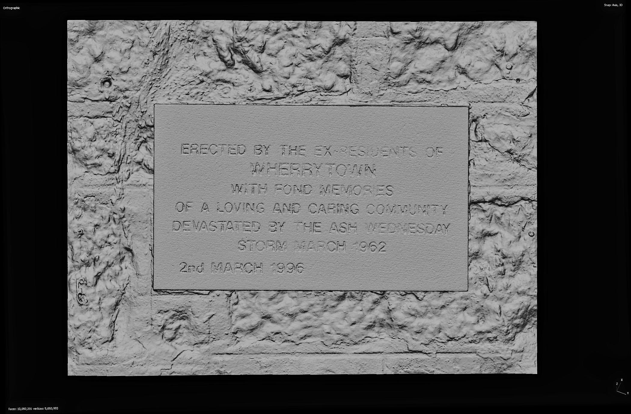 Source: Objaverse 1.0 / Sketchfab
Statue The Sign Of Law
Defending a [Non Molestation Order Defense](https://www.incourt.co.uk/post/can-you-appeal-a-non-molestation-order) requires the intricate gathering of evidence and may involve taking statements from witnesses as well as gathering other evidence regarding your character and behaviour. It is important that as soon as you are served with a Non-Molestation Order that you obtain expert legal advice quickly. Source: Objaverse 1.0 / Sketchfab
Green Dragon Tavern Sign
Sculpt based on an engraving of the original Green Dragon Tavern signage. https://www.thingiverse.com/thing: Source: Objaverse 1.0 / Sketchfab
Indices and sign arrays for floretion multiplication up to order 8.
<div> <div> <div> <p>A floretion is a type of hypercomplex number that extends the concept of quaternions. One main characteristic of floretions is their representation in an octal number system, where the digits are limited to {1, 2, 4, 7} which, when endowed with multiplication, become a discrete mathematical group. The number of digits in octal is the "order" of the group. These numbers can be associated with geometric shapes, specifically equilateral triangles, which are used to represent complex operations and properties visually.</p> <p>In mathematical operations, floretions employ logic operations like XOR for multiplication, following rules akin to quaternion multiplication but extended into higher dimensions and complexity. Floretions can be manipulated algebraically or graphically, each method offering unique insights into their structure and behavior.</p> <p>The development and use of floretions incorporate both algebraic structures and geometric representations, bridging a unique connection between number theory and visual geometry.</p> <p><a title="Floretion Calculator " href="https://floretions.com/">Floretion Calculator: floretions.com</a></p> <p><a href="https://github.com/Floretion-Inquisitor/floretions">Floretions at GitHub</a></p> <p> </p> <p> </p> </div> </div> </div> <p><strong>Dataset Description for Floretion Multiplication (up to order 8):</strong></p> <p>This collection of datasets, stored in numpy binary format, is designed to facilitate efficient multiplication of floretions up to order 8. The matrices included—indices and signs—are optimized for rapid computation of the product <strong>z=x⋅y</strong> using standard dot products, enhancing both speed and efficiency.</p> <p>For a foundational understanding, consider quaternion multiplication (order 1 floretions):</p> <h3>x = x[0]i + x[1]j + x[2]k + x[3]e </h3> <h3>y = y[0]i + y[1]j + y[2]k + y[3]e<code><br></code></h3> <p><strong>Multiplication Outcome</strong>: The coefficient for base vector "<strong>i</strong>" in <strong>z=x⋅y</strong> is calculated as:</p> <div><code>x[0]y[3]+x[1]y[2]−x[2]y[1]+x[3]y[0]=np.dot(np.multiply([1,−1,1,1],[x[3],x[2],x[1],x[0]]),[y[0],y[1],y[2],y[3]])</code></div> <p>Notice that <code>[1,−1,1,1]</code> above is the first row in the "signs" matrix and the indices of the coefficients of <strong>x</strong> are given by the first row of the "indices" matrix, below. </p> <h3>"Signs" Matrix<br>[[ 1 -1 1 1]<br>[ 1 1 -1 1]<br>[-1 1 1 1]<br>[-1 -1 -1 1]]</h3> <h3>"Indices" Matrix<br>[[3 2 1 0]<br>[2 3 0 1]<br>[1 0 3 2]<br>[0 1 2 3]]</h3> <p>These precomputed matrices streamline the computation of floretion products across various orders. For order 7 floretions, the data is split into 4 segments, for order 8 into 64 segments to keep file sizes managable. </p> <p> </p> <ul> <li> <div> <ul> <li> </li> </ul> </div> </li> </ul> <p> </p> <p> </p> <p> </p>
Supplementary materials for "Phonetic differences between affirmative and feedback head nods in German Sign Language (DGS): A pose estimation study"
<div> <pre>This is the supplementary data for the article "Phonetic differences between affirmative and feedback head nods in German Sign Language (DGS): A pose estimation study" by Anastasia Bauer, Anna Kuder, Marc Schulder and Job Schepens.<br><br>The supplementary data consists of three components, stored in separate directories:<br>- <code>annotations/</code>: The manual annotations of head nod categories, produced by Anna Kuder and Anastasia Bauer.<br>- <code>pose_analysis/</code>: Code and input/output files for the pose-based automatic analysis of phonetic attributes head nods, produced by Marc Schulder.<br>- <code>statistical_analysis/</code>: Code for the statistical analysis of the other two components and for the creation of related figures, produced by Job Schepens.<br><br>For further details, see the README files of the respective directories.</pre> </div>
Data for paper "Investigating the sign of stratocumulus adjustments to aerosols in the global storm-resolving model ICON"
<p>Data for paper "Investigating the sign of stratocumulus adjustments to aerosols in the global storm-resolving model ICON". The code used to generate, analyze and plot these data is provided separately on Zenodo. The zip files named 2.zip_file_name are used in the 2.make_comparison_plots notebooks in the companion Zenodo software repository. The zip files named 3.zip_file_name are generated using the code contained in 1.process_data in the software repository and used for the analyses in 3.calculate_causal_effects in the software repository. </p> <p><strong>References - Code ______________________________________________</strong></p> <p>J. Runge et al. (2015): Identifying causal gateways and mediators in complex spatio-temporal systems. Nature Communications, 6, 8502. <a href="http://doi.org/10.1038/ncomms9502">http://doi.org/10.1038/ncomms9502</a></p> <p>J. Runge, Necessary and sufficient graphical conditions for optimal adjustment sets in causal graphical models with hidden variables, Advances in Neural Information Processing Systems, 2021, 34. <a href="https://proceedings.neurips.cc/paper/2021/hash/8485ae387a981d783f8764e508151cd9-Abstract.html">https://proceedings.neurips.cc/paper/2021/hash/8485ae387a981d783f8764e508151cd9-Abstract.html</a></p> <p><strong>References - Data ______________________________________________</strong></p> <p><em>SEVIRI</em> <br>Benas, N., Solodovnik, I., Stengel, M., Hüser, I., Karlsson, K.-G., Håkansson, N., Johansson, E., Eliasson, S., Schröder, M., Hollmann, R., and Meirink, J. F.: CLAAS-3: The Third Edition of the CM SAF Cloud Data Record Based on SEVIRI Observations, Earth System , Science Data Discussions, pp. 1-38, <a href="https://doi.org/10.5194/essd-2023-79">https://doi.org/10.5194/essd-2023-79</a>, 2023.</p> <p><em>GOES</em><br>Walther, A. and Straka, W.: Algorithm Theoretical Basis Document For Daytime Cloud Optical and Microphysical Properties (DCOMP), 2020</p> <p><em>ERA5</em><br>Hersbach, H., Bell, B., Berrisford, P., Biavati, G., Horányi, A., Muñoz Sabater, J., Nicolas, J., Peubey, C., Radu, R., Rozum, I., Schepers, D., Simmons, A., Soci, C., Dee, D., and Thébaut, J.-N.: ERA5 Hourly Data on Single Levels from 1959 to Present, Copernicus Climate Change Service (C3S) Climate Data Store (CDS), <a href="https://doi.org/10.24381/cds.adbb2d47">https://doi.org/10.24381/cds.adbb2d47</a>, 2018a.<br>Hersbach, H., Bell, B., Berrisford, P., Biavati, G., Horányi, A., Muñoz Sabater, J., Nicolas, J., Peubey, C., Radu, R., Rozum, I., Schepers, D., Simmons, A., Soci, C., Dee, D., and Thébaut, J.-N.: ERA5 Hourly Data on Pressure Levels from 1959 to Present, Copernicus Climate Change Service (C3S) Climate Data Store (CDS), <a href="https://doi.org/10.24381/cds.bd0915c6">https://doi.org/10.24381/cds.bd0915c6</a>, 2018b.</p> <p><em>GPM</em><br>Huffman, G., Stocker, E., Bolvin, D., Nelkin, E., and Tan, J.: GPM IMERG Final Precipitation L3 Half Hourly 0.1 Degree x 0.1 Degree V07, Greenbelt, MD, Goddard Earth Sciences Data and Information Services Center (GES DISC), <a href="https://doi.org/10.5067/GPM/IMERG/3B-HH/07">https://doi.org/10.5067/GPM/IMERG/3B-</a><a href="https://doi.org/10.5067/GPM/IMERG/3B-HH/07">HH/07</a>, 2023</p> <p><em>MODIS</em><br>Platnick, S. et al. MODIS atmosphere L3 daily product. NASA<a href="https://doi.org/10.5067/MODIS/MOD08_D3.006"> https://doi.org/10.5067/MODIS/MOD08_D3.006 </a>, 2015.</p> <p><em>MIDAS</em><br>Eastman, R., McCoy, I. L., Schulz, H., and Wood, R.: A Survey of Radiative and Physical Properties of North Atlantic Mesoscale Cloud Morphologies from Multiple Identification Methodologies, EGUsphere, pp. 1–33, <a href="https://doi.org/10.5194/egusphere-2023-2118">https://doi.org/10.5194/egusphere-2023-2118</a>, 2023. <br>McCoy, I. L., McCoy, D. T., Wood, R., Zuidema, P., and Bender, F. A.-M.: The Role of Mesoscale Cloud Morphology in the Shortwave Cloud Feedback, Geophysical Research Letters, 50, e2022GL101 042, <a href="https://doi.org/10.1029/2022GL101042">https://doi.org/10.1029/2022GL101042</a>, 2023.</p> <p><em>ICON</em><br>Zängl, G., Reinert, D., Rípodas, P., and Baldauf, M.: The ICON (ICOsahedral Non-hydrostatic) Modelling Framework of DWD and MPI-M: Description of the Non-Hydrostatic Dynamical Core, Quarterly Journal of the Royal Meteorological Society, 141, 563–579, <a href="https://doi.org/10.1002/qj.2378">https://doi.org/10.1002/qj.2378</a>, 2015<br><a href="https://code.mpimet.mpg.de/projects/iconpublic/wiki/Instructions_to_obtain_the_ICON_model_code_with_a_personal_non-commercial_research_license">https://code.mpimet.mpg.de/projects/iconpublic/wiki/Instructions_to_obtain_the_ICON_model_code_with_a_personal_non-commercial_research_license </a></p>
DC-SIGN expression on myeloid population in Luminal Breast Cancer
<p>DC-SIGN expression by the different populations of DC and macrophages found in breast tumor samples using flow cytometry. As previously described (doi:10.1038/s41590-018-0145-8.), we identified four major DC populations: CD11c − CD123+ plasmacytoid pre-DCs, CD11c+BDCA1+ CD14− DCs, CD11c+ BDCA1− CD14− DCs, and CD11c+ BDCA1+ CD14+ inflammatory DCs. Staining was performed using the following antibodies: anti-CD45 APC-Cy7 (BD), anti-CD14 Qdot 605 (Thermo), anti-CD3 Alexa700 (Biolegend), anti-CD 19 Alexa700 (Biolegend), anti-CD56 Alexa700 (Biolegend), 400 anti-HLA-DR BV711 (Biolegend), anti-CD11c PC5 (Beckman Coulter), anti-BDCA-1 PE (BD), anti-CD123 PCy7 (BD) and anti-C-SIGN FITC (BD). Cells were analyzed by a LSRFORTESSA X-20 instrument (BD Biosciences). The most prominent intratumoral myeloid cell population, however, was shown to be represented by macrophages, defined as CD11c+ BDCA1−CD14+ cells. We analyzed DC-SIGN expression on the surface of these populations by flow cytometry. DC-SIGN was only expressed on the membrane of macrophages from tumoral as well as juxtatumoral tissues, but not on the DC populations analyzed. These results are represented in Figure 4 from the publication "Aberrant fucosylation enables breast cancer clusterin to interact with dendritic cell-specific ICAM-grabbing non-integrin (DC-SIGN)". </p> <p> </p>
lingpy/sign-language-evolution-paper: Evolutionary Dynamics in the Dispersal of Sign Languages
<p>Supplement for study on Manual Alphabet evolution.</p>
What is CoARA, what does signing mean, and what does it not mean?
<p>Presentation given at the UK CoARA National Chapter meeting on 8th October 2024. This presentation gives an overview of CoARA, discusses some of the implications of signing the Agreement on Reforming Research Assessment and busts some myths related to CoARA. A copy of the slides is also attached. </p>
ScienceDex guides
Understand access before you commit
These curated guides explain access requirements, typical timelines, costs, and reuse considerations for widely used research datasets.
Allen Brain Atlas
Allen Brain Atlas is an Allen Institute collection of brain map atlases, datasets, APIs, and analysis tools covering mouse, human, and non-human primate brain resources.
Annotated Behaviour and Observability Dataset (ABODe)
ABODe is a University of Edinburgh DataShare dataset for behavior classification in group-housed mice using home-cage video, identities, bounding boxes, ground-plate positions, and annotator labels.
DANDI Archive for NWB datasets
DANDI is a BRAIN Initiative archive for publishing and sharing neurophysiology data, including electrophysiology, optophysiology, and behavioral data packaged as NWB and related standards.
International Brain Laboratory public data
The International Brain Laboratory public data releases expose standardized mouse decision-making experiments, including Neuropixels recordings, widefield calcium imaging, behavior, and session metadata accessed through the ONE API.
OpenNeuro
OpenNeuro is a free, open platform for sharing neuroimaging datasets, with public search, dataset pages, and download paths for web, S3, DataLad, and the OpenNeuro CLI.