


Fluorescence spectrophotometry is a set of techniques that deals with the measurement of fluorescence emitted by substances when exposed to ultraviolet, visible, or other electromagnetic radiation.
It has wide application in chemical and biological sciences as it can be used to analyze a biological system, by studying its interactions with fluorescent probe molecules (So and Dong, 2002, The International Pharmacopoeia, 2019).
In the literature, the terms fluorescence spectrophotometry, fluorescence spectroscopy, fluorometry, and spectrofluorometry are often used interchangeably.
Fluorescence spectrophotometry is based on fluorescence, which is a photoluminescence event (photo = light; luminescence = the emission of light). In simple terms, it is the emission of light because of exposure to (and resultant absorption of) light.
Here, this exposure to and absorption of light is called excitation. A common form in which photoluminescence is often observed, is as phosphorescence – what you see in glow-in-the-dark toys.
This type of photoluminescence occurs when there is a long delay between the excitation and emission of light.
A long delay here means about 10-6 seconds or longer. When the delay between excitation and emission is shorter (between 10-6 and 10-8 seconds), the result is fluorescence (Wouterlood and Boekel, 2009).
Phosphorescence can persist long after the initial exposure to light – hence you may see the glow-in-the-dark star against your bedroom ceiling even after the room had been dark for hours.
Fluorescence, on the other hand, has a quick flash of emission (typically around 10 nanoseconds, but sometimes shorter than 1 nanosecond). Because of this, sophisticated electronics and optics are nowadays used to detect and measure fluorescence (Lakowicz, 2013).
The first observation and description of fluorescence, however, was done with little more than a glass of tonic water, sunlight, and the human eye. The human whose eye that was, is Sir John Frederick William Herschel (1792 – 1871).
In 1845, he reported on this phenomenon. He mixed equal amounts of quinine and tartaric acid in water, diluted it, poured it into a glass cylinder, and looked at it from all angles, where it stood by a window in bright sunlight.
What he saw was “an extremely vivid and beautiful celestial blue color” (Herschel, 1845). The celestial blue color came from the aromatic organic molecule (or fluorophore), quinine, present in tonic water.
The physics behind fluorescence involves the different electronic and vibrational states that fluorophores can exist in. An electronic state is divided into multiple vibrational states.
Photons, that have energies in the ultraviolet to a blue-green range of the spectrum can trigger an electronic transition from the lowest vibration in the ground state to one of the vibrational levels in a higher electronic excited state (So and Dong, 2002).
As soon as the energy input from the photon (in other words the excitation) stops, the fluorophore molecule relaxes into the lowest vibrational level of the excited electronic state.
The fluorophore remains in this state for some time (around 10 nanoseconds, known as the fluorescence lifetime) and then returns to the electronic ground state. This return to the ground state is associated with a release of energy, known as fluorescence emission (So and Dong, 2002).
The number of photons emitted by a fluorophore, relative to the number of photons absorbed, is called the quantum yield. A fluorophore with a large quantum yield, like rhodamine, will display a bright emission.
The emitted radiation is always of a longer wavelength (lower energy) than the excitation radiation (higher energy). For example, if the incoming light was blue (shorter wavelength), then the appropriate fluorophore will emit green light (longer wavelength).
This observation, which was first described by Sir George Gabriel Stokes, and therefore today called the Stokes shift, is caused by the rapid return of the excited molecule to its ground state (Lakowicz, 2013, Wouterlood and Boekel, 2009).
The process that happens between excitation and emission is illustrated using Jablonski diagrams (named after the father of fluorescence spectroscopy, Alexander Jablonski) (Lakowicz, 2013). These diagrams, such as the one in figure 1, show the different electronic (S0 and S1) and vibrational (0,1,2,3) states of a molecule.
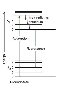
Figure 1. Jablonski diagram (Jacobkhed, 2002 [CC0 1.0])
Intrinsic fluorophores are molecules with a natural fluorescence, such as chlorophyll and aromatic amino acids.
Extrinsic fluorophores are those that are added to a sample to provide fluorescence, or to change the spectral properties of the sample. Examples of extrinsic fluorophores are fluorescein and rhodamine, but there are many more (Lakowicz, 2013).
Each fluorophore has its own characteristic properties, such as fluorescence lifetime, intensity, and position of the emission wavelength, thus, each fluorophore will yield a unique fluorescence spectrum. A fluorescence spectrum is a plot of the fluorescence intensity as a function of wavelength (Albani, 2007).
The environment in which the fluorophore finds itself will influence and modify its properties, hence reading the fluorescence spectrum of a fluorophore when immersed in different environments will give information about those environments (Albani, 2007, Lakowicz, 2013).
For example, the intrinsic fluorophore tryptophan is an aromatic amino acid that is very sensitive to its local environment within the cell. When a ligand binds to it, or when it associates with a protein, or when a protein unfolds, tryptophan’s fluorescence spectrum will change in particular ways.
By monitoring this change in the spectrum, one can deduce information about the immediate cellular and molecular environment.
In this way fluorophores, when linked to peptides, proteins, membranes, or DNA, can be used to study the structure, dynamics, and metabolism of living cells (Albani, 2007).
While some fluorescence can be detected with the eye, sophisticated instruments have been built to detect even the faintest fluorescence emitted by a molecule.
An older type of instrument for the measurement of fluorescence spectra, and one that is still used today, is the filter fluorometer. It consists of the following parts:
The filters only permit radiation of certain wavelengths (typically the primary filter permits short wavelengths needed for excitation and the secondary filter permits long wavelengths associated with emission) and serves to eliminate residual radiation scatter.
The fluorescence detection system consists of photomultiplier tubes (PMT) that amplify the photon emission and record and display the signal electronically (Albani, 2007, Sharma and Shulman, 1999, The International Pharmacopoeia, 2019).
Most modern fluorescence spectrophotometers (also called spectrofluorometers) are more advanced instruments than the filter fluorometer in that they can detect fluorescence with higher precision and extraordinary sensitivity.
They are superior in wavelength selectivity, flexibility, and convenience. A spectrofluorometer (see figure 2) is often equipped with the following:
The high-pressure xenon arc lamp, used as the excitation source, can provide an energy continuum that extends from the ultraviolet into the infrared (The International Pharmacopoeia, 2019).
Instead of filters, spectrofluorometers have monochromators that allow for the production of individual wavelengths from a broad-band light source (Sharma and Shulman, 1999). This makes it possible for spectrofluorometers to record both excitation and emission spectra (Lakowicz, 2013).
The monochromators allow one to keep emission fixed at a single wavelength to obtain the excitation spectrum. Vice versa, it is possible to keep excitation fixed at a single wavelength, to record the fluorescence emission spectrum (Albani, 2007, Lakowicz, 2013).
Like the fluorometer, the spectrofluorometer’s fluorescence detection system consists of photomultiplier tubes (PMT) for emission amplification. Electronic devices are then used to quantify the signal and display it electronically, usually as a graph (Lakowicz, 2013).
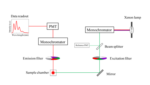
Figure 2. Schematic diagram of a spectrofluorometer (Sobarwiki, 2013 [Public domain])
Fluorescent measurements can be classified into:
In steady-state measurements, a sample is illuminated with a continuous beam of light and the fluorescence intensity of fluorescence emission spectrum is recorded.
In time-resolved measurements, a sample is illuminated by a short pulse of light after which the intensity decay or anisotropy decay is measured. (Lakowicz, 2013). Intensity decay refers to the fluorescence lifetime or the time that a molecule spends in the excited electronic state.
How long the molecule’s fluorescence lifetime is can provide rich information about the environment surrounding the fluorophore (Sharma and Shulman, 1999).
From the basic technology of fluorescence detection, as outlined above, a plethora of fluorescence technologies have evolved, such as multiphoton excitation, fluorescence correlation spectroscopy, single-molecule detection, fluorescence immunoassay, flow cytometry, and near-infrared fluorescence spectroscopy (Lakowicz, 2013, Sharma and Shulman, 1999).
The applications of fluorescence spectroscopy are almost as wide as one’s imagination. It is hard to imagine the chemical and biological sciences without this technique nowadays.
Only selected examples of application per sector, for some of the most common sectors it is used in, will be mentioned in the quick overview that follows.
In biosciences, one of the most frequent applications of fluorescence spectroscopy is the high precision quantification of DNA and RNA. An extrinsic fluorophore (often ethidium bromide) is added to a DNA sample and the sample is loaded into a fluorescence spectrometer to obtain a reading of the sample’s concentration.
Another modern application is SMRT (single molecule real-time) DNA sequencing. In its ability to produce long-read single molecules with high accuracy, it is predicted to be central to the next genetic diagnostic revolution (Ardui et al, 2018).
Fluorescence spectroscopy is used in several industrial settings as a fast, non-invasive technique in the assessment of contamination (Kohli, 2012). For example, it has been used to detect contaminating organic compounds in groundwater, after hydraulic fracturing for gas exploration (Dahm et al., 2011).
An important chemical application of fluorescence spectroscopy can be found in the field of nanoparticle synthesis for potential medical uses, such as drug delivery.
When nanoparticles are exposed to biological fluids, they become coated with proteins and other biomolecules (called the protein corona). The interactions between the nanoparticle and the protein corona have implications for its safe use in vivo.
Time-resolved fluorescence quenching and fluorescence correlation spectroscopy are used to study these interactions and understand nanotechnology better (Röcker et al., 2009).
In environmental monitoring, the technique also has wide application. One example is in the treatment of water surrounding landfill areas.
As rainwater percolates through waste and liquid forms during the biodegradation of waste in a landfill, landfill leachates form. Leachate contains a mix of pollutants that can be harmful to the environment.
High-resolution fluorescence spectroscopy and 3D-excitation emission matrix fluorescence spectroscopy are used to characterize dissolved organic matter in these samples and then based on that, optimize treatment processes for landfill leachate (Leenheer and Croué, 2003, Zhang et al., 2013).
Spectrofluorometric techniques are also used in the pharmaceutical field to analyze drugs. An example is the analysis of co-formulated tablets prescribed as cholesterol medication.
Synchronous fluorescence spectroscopy provides a simple, fast, and accurate method for analyzing a tablet called Atoreza©, which contains both Ezetimibe and Atorvastatin calcium. The method is ideal for routine quality control of this medication (Ayad and Magdy, 2015).
In agriculture, spectroscopic techniques are also widely applied for instance in the identification of different crop varieties. The laser-induced fluorescent emission technique (LIFS) is an excellent tool used to identify citrus seedling varieties (Milori et al., 2013).
Likewise, total luminescence spectroscopy can be used by tea manufacturers as a quick, affordable, and objective alternative to employing trained tea tasters, to discriminate between similar types of tea (Seetohul et al., 2013).
As fluorescence spectrophotometry spans a history of nearly 70 years, it has evolved into a technique with numerous sophisticated uses.
Any particular situation where it can be applied thus warrants careful research into the most suitable way in which it can be used to obtain the needed outcomes.
Fortunately, a wealth of literature and commercial options are available for scientists wanting to explore fluorescence spectrophotometry in greater depth.
In behavioral neuroscience, the Open Field Test (OFT) remains one of the most widely used assays to evaluate rodent models of affect, cognition, and motivation. It provides a non-invasive framework for examining how animals respond to novelty, stress, and pharmacological or environmental manipulations. Among the test’s core metrics, the percentage of time spent in the center zone offers a uniquely normalized and sensitive measure of an animal’s emotional reactivity and willingness to engage with a potentially risky environment.
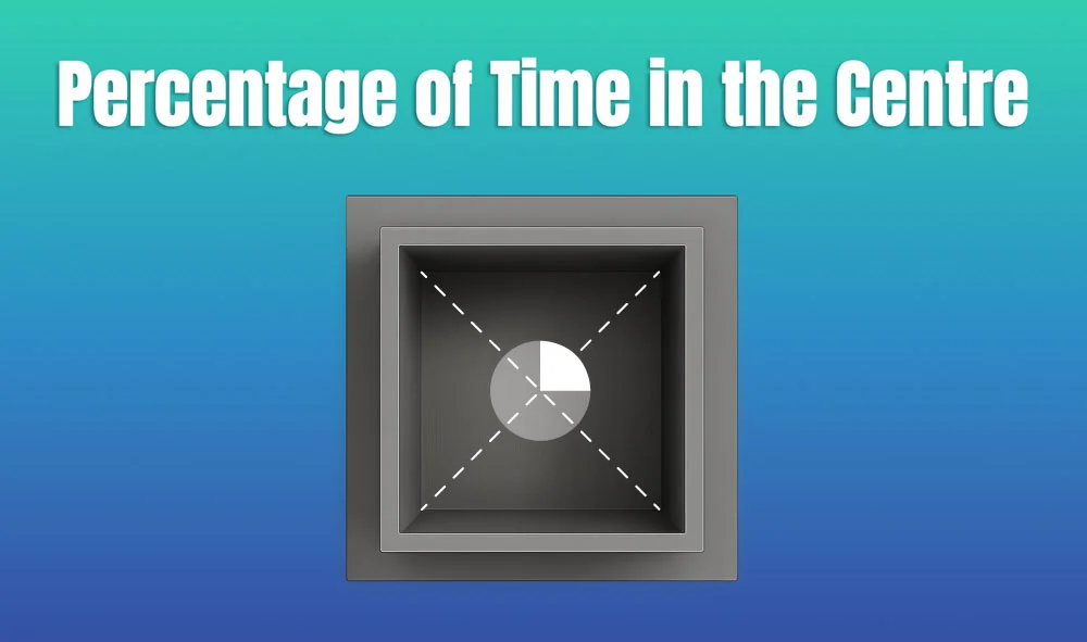
This metric is calculated as the proportion of time spent in the central area of the arena—typically the inner 25%—relative to the entire session duration. By normalizing this value, researchers gain a behaviorally informative variable that is resilient to fluctuations in session length or overall movement levels. This makes it especially valuable in comparative analyses, longitudinal monitoring, and cross-model validation.
Unlike raw center duration, which can be affected by trial design inconsistencies, the percentage-based measure enables clearer comparisons across animals, treatments, and conditions. It plays a key role in identifying trait anxiety, avoidance behavior, risk-taking tendencies, and environmental adaptation, making it indispensable in both basic and translational research contexts.
Whereas simple center duration provides absolute time, the percentage-based metric introduces greater interpretability and reproducibility, especially when comparing different animal models, treatment conditions, or experimental setups. It is particularly effective for quantifying avoidance behaviors, risk assessment strategies, and trait anxiety profiles in both acute and longitudinal designs.
This metric reflects the relative amount of time an animal chooses to spend in the open, exposed portion of the arena—typically defined as the inner 25% of a square or circular enclosure. Because rodents innately prefer the periphery (thigmotaxis), time in the center is inversely associated with anxiety-like behavior. As such, this percentage is considered a sensitive, normalized index of:
Critically, because this metric is normalized by session duration, it accommodates variability in activity levels or testing conditions. This makes it especially suitable for comparing across individuals, treatment groups, or timepoints in longitudinal studies.
A high percentage of center time indicates reduced anxiety, increased novelty-seeking, or pharmacological modulation (e.g., anxiolysis). Conversely, a low percentage suggests emotional inhibition, behavioral avoidance, or contextual hypervigilance. reduced anxiety, increased novelty-seeking, or pharmacological modulation (e.g., anxiolysis). Conversely, a low percentage suggests emotional inhibition, behavioral avoidance, or contextual hypervigilance.
The percentage of center time is one of the most direct, unconditioned readouts of anxiety-like behavior in rodents. It is frequently reduced in models of PTSD, chronic stress, or early-life adversity, where animals exhibit persistent avoidance of the center due to heightened emotional reactivity. This metric can also distinguish between acute anxiety responses and enduring trait anxiety, especially in longitudinal or developmental studies. Its normalized nature makes it ideal for comparing across cohorts with variable locomotor profiles, helping researchers detect true affective changes rather than activity-based confounds.
Rodents that spend more time in the center zone typically exhibit broader and more flexible exploration strategies. This behavior reflects not only reduced anxiety but also cognitive engagement and environmental curiosity. High center percentage is associated with robust spatial learning, attentional scanning, and memory encoding functions, supported by coordinated activation in the prefrontal cortex, hippocampus, and basal forebrain. In contrast, reduced center engagement may signal spatial rigidity, attentional narrowing, or cognitive withdrawal, particularly in models of neurodegeneration or aging.
The open field test remains one of the most widely accepted platforms for testing anxiolytic and psychotropic drugs. The percentage of center time reliably increases following administration of anxiolytic agents such as benzodiazepines, SSRIs, and GABA-A receptor agonists. This metric serves as a sensitive and reproducible endpoint in preclinical dose-finding studies, mechanistic pharmacology, and compound screening pipelines. It also aids in differentiating true anxiolytic effects from sedation or motor suppression by integrating with other behavioral parameters like distance traveled and entry count (Prut & Belzung, 2003).
Sex-based differences in emotional regulation often manifest in open field behavior, with female rodents generally exhibiting higher variability in center zone metrics due to hormonal cycling. For example, estrogen has been shown to facilitate exploratory behavior and increase center occupancy, while progesterone and stress-induced corticosterone often reduce it. Studies involving gonadectomy, hormone replacement, or sex-specific genetic knockouts use this metric to quantify the impact of endocrine factors on anxiety and exploratory behavior. As such, it remains a vital tool for dissecting sex-dependent neurobehavioral dynamics.
The percentage of center time is one of the most direct, unconditioned readouts of anxiety-like behavior in rodents. It is frequently reduced in models of PTSD, chronic stress, or early-life adversity. Because it is normalized, this metric is especially helpful for distinguishing between genuine avoidance and low general activity.
Environmental Control: Uniformity in environmental conditions is essential. Lighting should be evenly diffused to avoid shadow bias, and noise should be minimized to prevent stress-induced variability. The arena must be cleaned between trials using odor-neutral solutions to eliminate scent trails or pheromone cues that may affect zone preference. Any variation in these conditions can introduce systematic bias in center zone behavior. Use consistent definitions of the center zone (commonly 25% of total area) to allow valid comparisons. Software-based segmentation enhances spatial precision.
Evaluating how center time evolves across the duration of a session—divided into early, middle, and late thirds—provides insight into behavioral transitions and adaptive responses. Animals may begin by avoiding the center, only to gradually increase center time as they habituate to the environment. Conversely, persistently low center time across the session can signal prolonged anxiety, fear generalization, or a trait-like avoidance phenotype.
To validate the significance of center time percentage, it should be examined alongside results from other anxiety-related tests such as the Elevated Plus Maze, Light-Dark Box, or Novelty Suppressed Feeding. Concordance across paradigms supports the reliability of center time as a trait marker, while discordance may indicate task-specific reactivity or behavioral dissociation.
When paired with high-resolution scoring of behavioral events such as rearing, grooming, defecation, or immobility, center time offers a richer view of the animal’s internal state. For example, an animal that spends substantial time in the center while grooming may be coping with mild stress, while another that remains immobile in the periphery may be experiencing more severe anxiety. Microstructure analysis aids in decoding the complexity behind spatial behavior.
Animals naturally vary in their exploratory style. By analyzing percentage of center time across subjects, researchers can identify behavioral subgroups—such as consistently bold individuals who frequently explore the center versus cautious animals that remain along the periphery. These classifications can be used to examine predictors of drug response, resilience to stress, or vulnerability to neuropsychiatric disorders.
In studies with large cohorts or multiple behavioral variables, machine learning techniques such as hierarchical clustering or principal component analysis can incorporate center time percentage to discover novel phenotypic groupings. These data-driven approaches help uncover latent dimensions of behavior that may not be visible through univariate analyses alone.
Total locomotion helps contextualize center time. Low percentage values in animals with minimal movement may reflect sedation or fatigue, while similar values in high-mobility subjects suggest deliberate avoidance. This metric helps distinguish emotional versus motor causes of low center engagement.
This measure indicates how often the animal initiates exploration of the center zone. When combined with percentage of time, it differentiates between frequent but brief visits (indicative of anxiety or impulsivity) versus fewer but sustained center engagements (suggesting comfort and behavioral confidence).
The delay before the first center entry reflects initial threat appraisal. Longer latencies may be associated with heightened fear or low motivation, while shorter latencies are typically linked to exploratory drive or low anxiety.
Time spent hugging the walls offers a spatial counterbalance to center metrics. High thigmotaxis and low center time jointly support an interpretation of strong avoidance behavior. This inverse relationship helps triangulate affective and motivational states.
By expressing center zone activity as a proportion of total trial time, researchers gain a metric that is resistant to session variability and more readily comparable across time, treatment, and model conditions. This normalized measure enhances reproducibility and statistical power, particularly in multi-cohort or cross-laboratory designs.
For experimental designs aimed at assessing anxiety, exploratory strategy, or affective state, the percentage of time spent in the center offers one of the most robust and interpretable measures available in the Open Field Test.
Written by researchers, for researchers — powered by Conduct Science.


Monday – Friday
9 AM – 5 PM EST
DISCLAIMER: ConductScience and affiliate products are NOT designed for human consumption, testing, or clinical utilization. They are designed for pre-clinical utilization only. Customers purchasing apparatus for the purposes of scientific research or veterinary care affirm adherence to applicable regulatory bodies for the country in which their research or care is conducted.