


Scanning Tunneling Microscopy, or STM, is a scanning probe technique. This means that the specimen is imaged by scanning a very sharp tip over its surface, while information about the shape or composition of the surface is collected based on interactions between the tip and the sample. This is unlike optical or electron microscopy, where a beam of light or electrons either passes through or reflects off the specimen.
The main advantage of scanning probe techniques is that they are extremely sensitive to height or composition variations on the surface, with some having the potential for even atomic-level resolution (< 0.1 nanometer). In fact, STM was the first technique which was able to distinguish individual atoms on a surface.[1] Its inventors were awarded the Nobel Prize in physics in 1986.
In STM, the interaction between the probe tip and the specimen consists of quantum tunneling of electrons. This is a process where electrons can cross over a barrier, in this case the empty space between the specimen and the probe.
This is because the location of an electron is not described by a fixed position, but by a cloud, where the electron may exist anywhere within the cloud. If the cloud of an electron extends across a barrier, the electron can cross over it by existing simultaneously on both sides of the barrier.
Electron tunneling can happen at distances < 3 nm, with a probability that is strongly dependent on distance, which gives STM its extreme sensitivity at short length scales.
This is a simplified explanation, and a full analysis of tunneling in specific cases requires determining the quantum wavefunction of the electron in the system,[2] through use of the Schrӧedinger equation or other formulations.
Electrons can tunnel either between the tip and the specimen, or vice versa, depending on the applied voltage. In either case, the rules of quantum tunneling require that the individual electron tunnels between an occupied energy state in one to the same, unoccupied state in the other.
A central idea in quantum physics is that electrons exist in materials in such discrete (or quantized) energy states. The process of tunneling is shown schematically in the figure below.
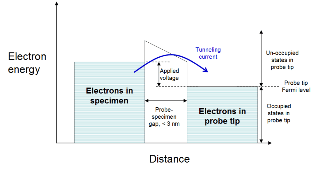
Figure: Schematic of the tunneling process.
The rate that electrons cross the barrier (or the tunneling current) depends on:
Tunneling current is roughly proportional to the first two, and depends exponentially on the third.[3]
In this article, we will first describe the various types of analysis that can be done with STM, based on the dependence of tunneling on these three factors. We will then discuss practical aspects of STM, including the parts of a typical STM setup, and considerations when performing experiments with an STM.
The three parameters that the STM analyst can vary and/or measure are the applied probe to specimen voltage, the probe height, and the tunneling current.[4] A number of different techniques can be built by varying these parameters. They are described below, from simplest to most complex.[5]
In this simple model, the probe is scanned (or rastered) in the x and y directions across the specimen. While the tip is being rastered, a voltage is applied to the specimen and the resulting tunneling current is measured.
An electronic feedback loop attempts to then keep this tunneling current constant during the x-y scanning by adjusting the z-position (height) of the probe tip. For example, if the tunneling current is higher than the set value, the feedback loop will retract the tip. Typical scan areas are in the ~ 100 to 10,000 nm2 range.
The resulting information is a two-dimensional x-y map of the probe height required to maintain a constant tunneling current, sometimes called a “topographic” map.
This height is a combination of the physical height variation of the surface, and the local density of electron states. The very strong exponential dependence of tunneling current on probe-specimen distance, however, results in high sensitivity to surface topography.
This mode is similar to the constant tunneling current mode, except that the tunneling current is measured, and the height of the probe tip is held constant.
The result in this case is a map of the tunneling current at constant height. As with constant current mode, the magnitude of the tunneling current depends on the shape of the surface, and the density of electron states.
The main advantage to constant height STM is that the tip can be scanned faster, since no feedback is needed. However, it requires an atomically flat specimen, and can only be used over small areas, since without feedback there is danger of having the probe contact the specimen.
A more sophisticated form of STM analysis involves varying or modulating either the probe to sample distance, or the applied voltage, during an x-y scan.
In the first case, the change in the tunneling current with probe to sample distance (dI/dz) is proportional to the local work function of the specimen.
The work function is the amount of energy required to remove an electron from a material, and depends on the composition and structure of the surface just under the probe tip.
In the second case, the change in tunneling current with applied voltage (dI/dV) is proportional to the local density of states in the material. So scanning in x-y while modulating the applied voltage can be used to map the density of states in the material, another useful diagnostic tool.
In the techniques of barrier height and density of states mapping, the height or voltage are continuously modulated during the x-y sweep. A more comprehensive analysis can be done where the probe stops at each point in the x-y scan, and runs a full sweep of probe height or supply voltage, measuring the resulting tunneling current response.
These are full I vs. Z and I vs. V curves. This type of scanning is much slower, but results in a full spectroscopic data set at each point, which can be useful when the response of the specimen is not easy to predict.
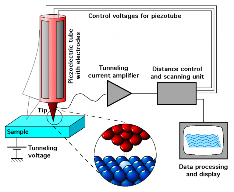
Figure: Schematic of an STM system.
Source: http://www.iap.tuwien.ac.at/www/surface/stm_gallery/stm_schematic
The probe tip is a critical part of the STM because it directly interacts with the specimen. The most critical aspect of the probe is the sharpness of the tip itself, which effectively determines the resolution of the image.
STM probes are traditionally metallic, specifically, either tungsten or platinum-iridium are common. They are formed by either mechanical methods, like shearing, or by electrochemical etching.[6] More recently, carbon nanotubes have been used.
The position of the tip in all three dimensions is typically controlled using piezoelectric transducers,[7] or simply “piezos”. These consist of crystals that expand or contract by minute amounts when voltage is applied. So by applying variable voltages to crystals controlling the x and y positions, the position of the probe tip can be scanned across the specimen.
Conversely, if the piezo crystals are compressed or put in tension, a voltage is generated across the crystal. So the position of the probe tip can also be sensed by measuring the voltage.
In an STM setup, the piezo crystals responsible for x and y motion are directly controlled by a computer. Z motion, which determines the probe height, has the additional capability or being controlled by a feedback loop in constant tunneling current measurements.
The electronics in an STM are straightforward but very sensitive and precise. First, a voltage source applies a small voltage to the specimen. When the probe is at a typical scanning distance (< 1 nm, or 10-9 m), a small tunneling current, on the order of 10-9 A, is generated. An amplifier converts this small current to a voltage, and this voltage signal is sent to control electronics.
Unlike electron microscopy, there is nothing inherent about the physics of the STM technique that requires special environmental conditions. However, since STM is surface-sensitive, a highly controlled environment is required to maintain surface cleanliness.
Consider that at 10-6 Torr, considered a moderately high vacuum, a gas molecule impacts every atom on a surface once per second. For that reason, STM analysis is normally performed under ultra-high vacuum conditions, which greatly reduces contamination from background gases.
However, STM can be performed in other controlled environments, including under the surface of liquids.[4]
Because the distances being measured in STM are extremely small, at times < 0.1 nm, the technique is very sensitive to vibrations, even more so than other microscopy techniques.
Even the imperceptible vibrations from a nearby road or other lab equipment can severely limit or even prevent the operation of an STM. For that reason, all components in the STM are designed to be rigid.
Furthermore, STM equipment must be isolated from vibrations by mounting it on dampening air springs or similar hardware. The placement of the STM in a building is also critical for this reason.
Analysis using STM is normally done with the assistance of a trained expert since these instruments are extremely sensitive and complicated to operate. Similar to TEM, one of the most difficult and critical aspects of the process is sample preparation. The quality of the analysis often depends on how well the sample was prepared.
Analysis by STM is highly dependent on the type of sample and the instrument being used. The steps given here are a rough generalization of the analysis method.
Scanning tunneling microscopes are expensive and sensitive pieces of equipment, so in most cases, they are owned and maintained by trained staff. For the individual users of an STM, there are a number of guidelines that will help to prevent damage to the equipment:
Scanning tunneling microscopes are quite different from the more common optical and electron microscopes, and the information they provide is different and often complementary to those instruments.
STM differs from those techniques mainly in its ability to provide detailed information on the atomic-level, local structure of the surface of a material, and extremely good resolution in the vertical (height) dimension. Because of this, STM is considered a surface science tool as well as a microscope.
STM is closely related to atomic force microscopy (AFM), which is also a scanning probe technique with good height resolution. The key difference between STM and AFM is that AFM uses intermolecular or interatomic forces, rather than quantum tunneling, to scan the surface.
The main drawbacks to STM are:
In behavioral neuroscience, the Open Field Test (OFT) remains one of the most widely used assays to evaluate rodent models of affect, cognition, and motivation. It provides a non-invasive framework for examining how animals respond to novelty, stress, and pharmacological or environmental manipulations. Among the test’s core metrics, the percentage of time spent in the center zone offers a uniquely normalized and sensitive measure of an animal’s emotional reactivity and willingness to engage with a potentially risky environment.
This metric is calculated as the proportion of time spent in the central area of the arena—typically the inner 25%—relative to the entire session duration. By normalizing this value, researchers gain a behaviorally informative variable that is resilient to fluctuations in session length or overall movement levels. This makes it especially valuable in comparative analyses, longitudinal monitoring, and cross-model validation.
Unlike raw center duration, which can be affected by trial design inconsistencies, the percentage-based measure enables clearer comparisons across animals, treatments, and conditions. It plays a key role in identifying trait anxiety, avoidance behavior, risk-taking tendencies, and environmental adaptation, making it indispensable in both basic and translational research contexts.
Whereas simple center duration provides absolute time, the percentage-based metric introduces greater interpretability and reproducibility, especially when comparing different animal models, treatment conditions, or experimental setups. It is particularly effective for quantifying avoidance behaviors, risk assessment strategies, and trait anxiety profiles in both acute and longitudinal designs.
This metric reflects the relative amount of time an animal chooses to spend in the open, exposed portion of the arena—typically defined as the inner 25% of a square or circular enclosure. Because rodents innately prefer the periphery (thigmotaxis), time in the center is inversely associated with anxiety-like behavior. As such, this percentage is considered a sensitive, normalized index of:
Critically, because this metric is normalized by session duration, it accommodates variability in activity levels or testing conditions. This makes it especially suitable for comparing across individuals, treatment groups, or timepoints in longitudinal studies.
A high percentage of center time indicates reduced anxiety, increased novelty-seeking, or pharmacological modulation (e.g., anxiolysis). Conversely, a low percentage suggests emotional inhibition, behavioral avoidance, or contextual hypervigilance. reduced anxiety, increased novelty-seeking, or pharmacological modulation (e.g., anxiolysis). Conversely, a low percentage suggests emotional inhibition, behavioral avoidance, or contextual hypervigilance.
The percentage of center time is one of the most direct, unconditioned readouts of anxiety-like behavior in rodents. It is frequently reduced in models of PTSD, chronic stress, or early-life adversity, where animals exhibit persistent avoidance of the center due to heightened emotional reactivity. This metric can also distinguish between acute anxiety responses and enduring trait anxiety, especially in longitudinal or developmental studies. Its normalized nature makes it ideal for comparing across cohorts with variable locomotor profiles, helping researchers detect true affective changes rather than activity-based confounds.
Rodents that spend more time in the center zone typically exhibit broader and more flexible exploration strategies. This behavior reflects not only reduced anxiety but also cognitive engagement and environmental curiosity. High center percentage is associated with robust spatial learning, attentional scanning, and memory encoding functions, supported by coordinated activation in the prefrontal cortex, hippocampus, and basal forebrain. In contrast, reduced center engagement may signal spatial rigidity, attentional narrowing, or cognitive withdrawal, particularly in models of neurodegeneration or aging.
The open field test remains one of the most widely accepted platforms for testing anxiolytic and psychotropic drugs. The percentage of center time reliably increases following administration of anxiolytic agents such as benzodiazepines, SSRIs, and GABA-A receptor agonists. This metric serves as a sensitive and reproducible endpoint in preclinical dose-finding studies, mechanistic pharmacology, and compound screening pipelines. It also aids in differentiating true anxiolytic effects from sedation or motor suppression by integrating with other behavioral parameters like distance traveled and entry count (Prut & Belzung, 2003).
Sex-based differences in emotional regulation often manifest in open field behavior, with female rodents generally exhibiting higher variability in center zone metrics due to hormonal cycling. For example, estrogen has been shown to facilitate exploratory behavior and increase center occupancy, while progesterone and stress-induced corticosterone often reduce it. Studies involving gonadectomy, hormone replacement, or sex-specific genetic knockouts use this metric to quantify the impact of endocrine factors on anxiety and exploratory behavior. As such, it remains a vital tool for dissecting sex-dependent neurobehavioral dynamics.
The percentage of center time is one of the most direct, unconditioned readouts of anxiety-like behavior in rodents. It is frequently reduced in models of PTSD, chronic stress, or early-life adversity. Because it is normalized, this metric is especially helpful for distinguishing between genuine avoidance and low general activity.
Environmental Control: Uniformity in environmental conditions is essential. Lighting should be evenly diffused to avoid shadow bias, and noise should be minimized to prevent stress-induced variability. The arena must be cleaned between trials using odor-neutral solutions to eliminate scent trails or pheromone cues that may affect zone preference. Any variation in these conditions can introduce systematic bias in center zone behavior. Use consistent definitions of the center zone (commonly 25% of total area) to allow valid comparisons. Software-based segmentation enhances spatial precision.
Evaluating how center time evolves across the duration of a session—divided into early, middle, and late thirds—provides insight into behavioral transitions and adaptive responses. Animals may begin by avoiding the center, only to gradually increase center time as they habituate to the environment. Conversely, persistently low center time across the session can signal prolonged anxiety, fear generalization, or a trait-like avoidance phenotype.
To validate the significance of center time percentage, it should be examined alongside results from other anxiety-related tests such as the Elevated Plus Maze, Light-Dark Box, or Novelty Suppressed Feeding. Concordance across paradigms supports the reliability of center time as a trait marker, while discordance may indicate task-specific reactivity or behavioral dissociation.
When paired with high-resolution scoring of behavioral events such as rearing, grooming, defecation, or immobility, center time offers a richer view of the animal’s internal state. For example, an animal that spends substantial time in the center while grooming may be coping with mild stress, while another that remains immobile in the periphery may be experiencing more severe anxiety. Microstructure analysis aids in decoding the complexity behind spatial behavior.
Animals naturally vary in their exploratory style. By analyzing percentage of center time across subjects, researchers can identify behavioral subgroups—such as consistently bold individuals who frequently explore the center versus cautious animals that remain along the periphery. These classifications can be used to examine predictors of drug response, resilience to stress, or vulnerability to neuropsychiatric disorders.
In studies with large cohorts or multiple behavioral variables, machine learning techniques such as hierarchical clustering or principal component analysis can incorporate center time percentage to discover novel phenotypic groupings. These data-driven approaches help uncover latent dimensions of behavior that may not be visible through univariate analyses alone.
Total locomotion helps contextualize center time. Low percentage values in animals with minimal movement may reflect sedation or fatigue, while similar values in high-mobility subjects suggest deliberate avoidance. This metric helps distinguish emotional versus motor causes of low center engagement.
This measure indicates how often the animal initiates exploration of the center zone. When combined with percentage of time, it differentiates between frequent but brief visits (indicative of anxiety or impulsivity) versus fewer but sustained center engagements (suggesting comfort and behavioral confidence).
The delay before the first center entry reflects initial threat appraisal. Longer latencies may be associated with heightened fear or low motivation, while shorter latencies are typically linked to exploratory drive or low anxiety.
Time spent hugging the walls offers a spatial counterbalance to center metrics. High thigmotaxis and low center time jointly support an interpretation of strong avoidance behavior. This inverse relationship helps triangulate affective and motivational states.
By expressing center zone activity as a proportion of total trial time, researchers gain a metric that is resistant to session variability and more readily comparable across time, treatment, and model conditions. This normalized measure enhances reproducibility and statistical power, particularly in multi-cohort or cross-laboratory designs.
For experimental designs aimed at assessing anxiety, exploratory strategy, or affective state, the percentage of time spent in the center offers one of the most robust and interpretable measures available in the Open Field Test.
Written by researchers, for researchers — powered by Conduct Science.


Monday – Friday
9 AM – 5 PM EST
DISCLAIMER: ConductScience and affiliate products are NOT designed for human consumption, testing, or clinical utilization. They are designed for pre-clinical utilization only. Customers purchasing apparatus for the purposes of scientific research or veterinary care affirm adherence to applicable regulatory bodies for the country in which their research or care is conducted.