


The structure of a molecule can be predicted using NMR spectroscopy. However, the interpretation of the signals in an NMR spectrum relies on several factors. One of the factors affecting the location of the peaks in an NMR spectrum is Chemical shift.
The location of the peaks is important in discovering how many protons there are in a molecule, as well as other information about the surrounding electronic environment.
In addition to knowing where the peaks are, on the chemical shift scale, and what influences the delta value, one must also consider the fact that the peaks in an NMR spectrum are not always a singlet. [1][2]
In fact, the interactions between different types of protons present in the molecule cause a single peak on an NMR spectrum to split into doublet, triplet, or multiplet, a phenomenon known as the spin-spin coupling.
There could also be other complex peak splitting patterns. The spin-spin coupling phenomenon, at its core, involves spinning nuclei.
A nucleus that has an odd number of protons spins along its axis. A proton has two possible spin states +1/2 or -1/2. In the absence of a magnetic field, these spins are quite random. In the presence of an external magnetic field, there is a tendency of the nuclei to align either with or against the magnetic field. [3][4]
The spins which are aligned with the external magnetic field have a lower energy state than the ones aligned against the magnetic field. The spin states and the energy levels are shown in the diagram below:
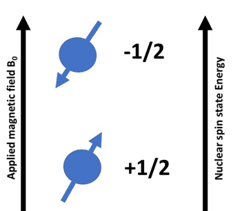
Depending on the orientation of the spins, the effective magnetic field on the proton would either increase or decrease by a small factor.
The applied magnetic field is denoted by B0
The induced magnetic field is denoted by Bi
The effective magnetic field experienced by the proton
Beff = B0– Bi
At the core of the molecule, these spinning nuclei ultimately give rise to the phenomenon of coupling in NMR spectrum.
The interaction between the spin magnetic moments of the different sets of H atoms in the molecule under study, is known as spin-spin coupling. It is imperative that a minimum of 2 sets of protons are present in adjacent positions.
The magnetic spins of these resonating nuclei interact with each other and affect each other’s precession frequencies.
The effective magnetic field (Beff) experienced by neighboring protons as a result of magnetic spins thereby affect the chemical shift values. [5] In addition to the chemical shifts, the nature of the peaks in the NMR spectrum is also affected.
A closer analysis of an NMR spectrum reveals that each signal on the graph represents one kind of proton present in the molecule. It is commonly observed that this signal is not always a single peak but has multiple peaks.
This multiplicity of the signal is a very important determinant for the structure of the molecule. This phenomenon by which the spins of resonating protons cause the peaks on the NMR spectrum to multiply is known as peak splitting. [6]
The splitting of the NMR signal gives precise information about the number of neighboring protons in a molecule. There is a formula to calculate the multiplicity of the peaks in the NMR spectrum.
2nI + 1
n= Number of neighboring protons
I= spin number of protons
Since I is always ½, we can rewrite the formula as n+1.
The other relevant information which comes along with knowing the number of peaks is the intensity of the peaks (which is seen as the height of the peaks).
As a general rule, the height of the peaks or in other words, the relative intensities of the peaks can be determined by using Pascal’s triangle. [7]
This is a number pattern invented by a famous French mathematician, Blaise Pascal. We can use the n+1 rule to determine the number of peaks.
The height of the peaks, caused due to spin-spin coupling is in proportion to the values in the row (corresponding to the value n) in Pascal’s triangle.
If we look at the figure below and consider a quartet, we would observe that the peak of the extreme signals is 1/3rd of the first and the last peak.
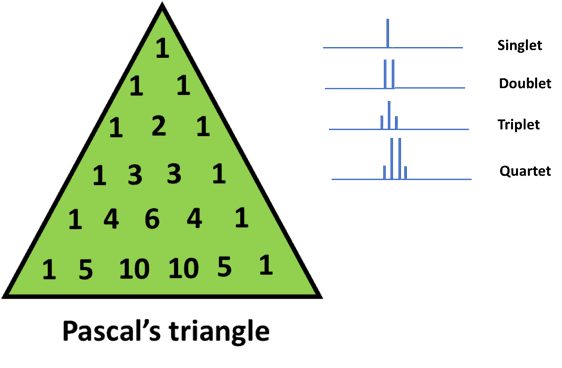
With n=0 (or 0 neighboring protons), we get a single peak. This is depicted as 1 at the apex of Pascal’s triangle
Similarly, for n=1 (or 1 neighboring proton), we get a doublet (using the n+1 rule). This is written as 1 on either side of the second row in Pascal’s triangle
Moving on, for n=2 (or 2 neighboring protons), we get a triplet. In this case, the number 1 is written at the left and right of the triangle and the sum (1+1) is shown in the middle.
For n=3, we get a quartet. In this case, again 1 is written at the ends and the neighboring numbers are added. Therefore, we end up with the sequence 1 3 3 1
We can explain the rest of Pascal’s triangle in a similar way. This method of generating numbers is known as binomial expansion.
Let us try to understand peak splitting using the following molecule as an example;
CH3CH2Cl (Ethyl chloride)
Let us calculate the multiplicity for the hydrogen atoms.
There are 2 sets of hydrogen atoms in Ethyl Chloride and we should expect to get 2 peaks in the NMR spectrum. This, however, is not true when it comes to visualizing the actual spectrum.
Each of the hydrogen atoms will influence the neighbors in an applied magnetic field and would lead to multiple peaks. To determine how many peaks we can get for hydrogen atoms in CH2 or CH3, we need to apply the above rule of multiplicity determination.
Let us look at the hydrogen atoms in CH2 which are under the influence of 3 hydrogen atoms of the CH3 group. Therefore,
n=3
I=1/2
After applying the formula,
2nI+1 = (2x3x1/2) + 1= 4
Therefore, there will be 4 peaks for hydrogen atoms in CH2
Similarly, there would be 3 peaks for hydrogen atoms in CH3
The position of the split peaks on the chemical shift scale (also known as the delta value) would be further influenced by the presence of the electronegative atom (chloride) in close proximity to hydrogen atoms in CH2
We have seen earlier that the nuclei have a property known as spin. The spinning hydrogen nuclei in a molecule will interact with each other and cause the signal in the NMR peak to split.
The separation distance between two adjacent peaks, as a result of the spin-spin interaction in a multiplet, is constant and is known as coupling constant (denoted by the letter J).
The value of the coupling constant depends on the following factors:
The distance between the hydrogen atoms in a molecule is an important determinant in the value of the J constant. If the hydrogen atoms involved in the coupling are closer to each other, these give rise to a greater value of the J constant than if these atoms are further apart.
The orientation or angle of the protons with respect to each other is equally important. The value of the J constant is greater in molecules, where the H atoms are in the cis conformation. Conversely, it is less when the H atoms are in the trans conformation.
Let us look at the interesting case of determining if the two adjacent peaks are doublets or actually made up of 2 singlets.
If we, for example, observe peaks in the molecule which are exactly 10 Hz apart and look indistinguishable from each other, it is very hard to decide if they are singlets or doublet.
Singlet/Doublet?
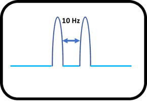
In order to know whether the peaks are a doublet, we would increase the applied magnetic field. Now, because the coupling constant (J) is constant between the adjacent peaks, the doublet peaks would be unaffected by the change of magnetic field. On the other hand, if the peaks were made of two singlets, then, the individual peaks would shift further apart on the chemical shift scale as shown below:

In the above example, if the peaks are doublets then the value of the coupling constant remains 10 Hz.
Unit of Coupling constant
The unit of a coupling constant is Hz and it is also referred as Cycles per second (CPS). The value of the coupling constant could be either positive or negative. The value of the coupling constant is a measure of interaction between neighboring protons.
When two spinning nuclei are in the opposite orientation then the energy is lower and the value of the constant is positive. However, if the spinning nuclei are in the same orientation, then, the energy is higher and the value of the constant is negative.
The spacing between the split lines or the J constant between coupling protons is of the same magnitude. The J constant can be used for distinguishing, e.g., between two singlets and one doublet or two doublet and one quartet. [8] There is no effect of the external magnetic field on the coupling constant.
Geminal coupling: The term Geminal means that 2 atoms or functional groups are bound to the same carbon atom. The geminal or 2-bond coupling constant is denoted by 2J. This also denotes that there are 2 bonds between the hydrogens being coupled.
In some cases, two hydrogen atoms can be attached to the same carbon atom but can be in a completely different electronic environment which gives rise to different chemical shifts. These protons are known as Geminal protons. Let us look at the molecule below:
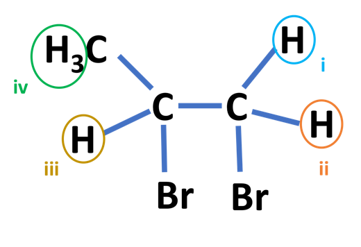
According to the definition of Geminal protons, protons I and II are geminal protons, as they are attached to the same carbon atom, however, their electronic environments are different.
The coupling constant value will also depend on the angle between protons I and II. The coupling constant will increase with the electronegativity of the groups. [9][10]
Vicinal Coupling: Vicinal protons are those which are separated by three bonds. In the molecule shown above, ii and iii are vicinal protons. The vicinal or 3 bond coupling constants are denoted by 3J. The hydrogen atoms are on the adjacent carbon atoms in vicinal coupling. [11][12]
Long range coupling: If the distance between two protons is more than 3 covalent bonds, then, the phenomenon of coupling does not come into play.
However, there would be some coupling if there are unsaturated or fluoro compounds present in the vicinity of the protons. Such type of coupling can only be observed using a very sensitive and high-resolution NMR spectrophotometer (e.g. the 600 MHz Bruker Avance Spectrometer). [13]
The NMR spectrum can sometimes have more complex splitting patterns than the simpler couplings involving equivalent coupling constants (such as doublet, triplet, quartet, quintet etc.).
It may sometimes happen that each peak in a doublet (in an NMR spectrum) is further split into another peak.
Such cases happen when a hydrogen atom is influenced by 2 adjacent non-equivalent hydrogen atoms. These complex patterns manifest as doublet of doublets, doublet of triplets, triplet of doublets etc. [14][15]
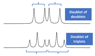
Let us investigate this effect using a molecule named methyl acrylate
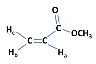
The protons Ha and Hb are coupled and would give rise to a doublet. The proton Hc is a non-equivalent proton and this would give rise to further splitting into a doublet of doublets.
It is important to note that Hc is coupled to both Ha and Hb but having different coupling constants. This is why each line in the doublet would further split into another doublet.
The resonating protons in a molecule are depicted as a series of peaks in the NMR spectrum. This physical interaction between the spinning nuclei is much more complex.
The nature of the peaks and the position on the chemical shift scale is dependent on the electronic environment and the phenomenon of spin-spin coupling comes into play. The peaks are further split due to factors such as bonds and bond angles.
The phenomenon of spin-spin coupling and the resulting coupling constant provides additional information which is very useful in elucidating the structure of the molecule under study.
Since this coupling constant, by definition, is a fixed value for the interacting nuclei, it does not change on different NMR machines. Although the coupling is independent of the applied magnetic field, it does diminish with an increase in the number of bonds between the interacting nuclei. [16]
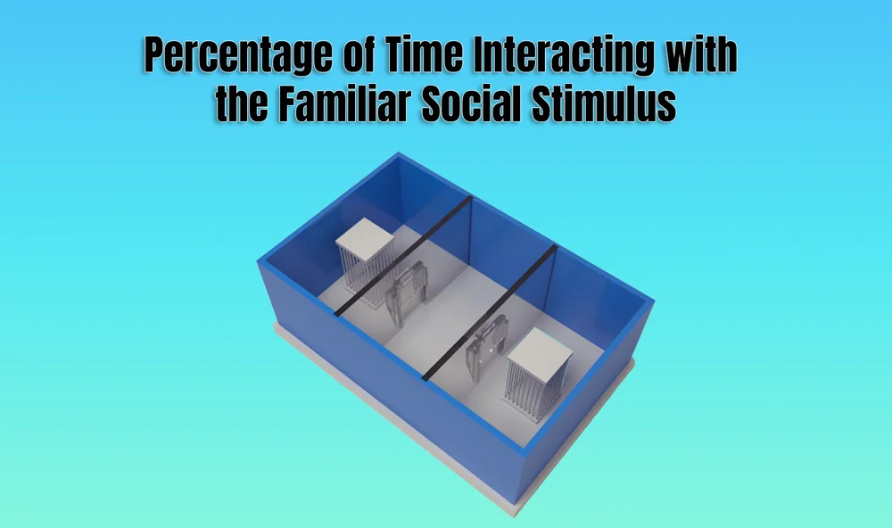
In behavioral neuroscience, the Open Field Test (OFT) remains one of the most widely used assays to evaluate rodent models of affect, cognition, and motivation. It provides a non-invasive framework for examining how animals respond to novelty, stress, and pharmacological or environmental manipulations. Among the test’s core metrics, the percentage of time spent in the center zone offers a uniquely normalized and sensitive measure of an animal’s emotional reactivity and willingness to engage with a potentially risky environment.
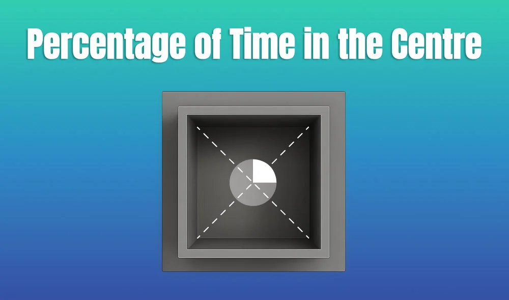
This metric is calculated as the proportion of time spent in the central area of the arena—typically the inner 25%—relative to the entire session duration. By normalizing this value, researchers gain a behaviorally informative variable that is resilient to fluctuations in session length or overall movement levels. This makes it especially valuable in comparative analyses, longitudinal monitoring, and cross-model validation.
Unlike raw center duration, which can be affected by trial design inconsistencies, the percentage-based measure enables clearer comparisons across animals, treatments, and conditions. It plays a key role in identifying trait anxiety, avoidance behavior, risk-taking tendencies, and environmental adaptation, making it indispensable in both basic and translational research contexts.
Whereas simple center duration provides absolute time, the percentage-based metric introduces greater interpretability and reproducibility, especially when comparing different animal models, treatment conditions, or experimental setups. It is particularly effective for quantifying avoidance behaviors, risk assessment strategies, and trait anxiety profiles in both acute and longitudinal designs.
This metric reflects the relative amount of time an animal chooses to spend in the open, exposed portion of the arena—typically defined as the inner 25% of a square or circular enclosure. Because rodents innately prefer the periphery (thigmotaxis), time in the center is inversely associated with anxiety-like behavior. As such, this percentage is considered a sensitive, normalized index of:
Critically, because this metric is normalized by session duration, it accommodates variability in activity levels or testing conditions. This makes it especially suitable for comparing across individuals, treatment groups, or timepoints in longitudinal studies.
A high percentage of center time indicates reduced anxiety, increased novelty-seeking, or pharmacological modulation (e.g., anxiolysis). Conversely, a low percentage suggests emotional inhibition, behavioral avoidance, or contextual hypervigilance. reduced anxiety, increased novelty-seeking, or pharmacological modulation (e.g., anxiolysis). Conversely, a low percentage suggests emotional inhibition, behavioral avoidance, or contextual hypervigilance.
The percentage of center time is one of the most direct, unconditioned readouts of anxiety-like behavior in rodents. It is frequently reduced in models of PTSD, chronic stress, or early-life adversity, where animals exhibit persistent avoidance of the center due to heightened emotional reactivity. This metric can also distinguish between acute anxiety responses and enduring trait anxiety, especially in longitudinal or developmental studies. Its normalized nature makes it ideal for comparing across cohorts with variable locomotor profiles, helping researchers detect true affective changes rather than activity-based confounds.
Rodents that spend more time in the center zone typically exhibit broader and more flexible exploration strategies. This behavior reflects not only reduced anxiety but also cognitive engagement and environmental curiosity. High center percentage is associated with robust spatial learning, attentional scanning, and memory encoding functions, supported by coordinated activation in the prefrontal cortex, hippocampus, and basal forebrain. In contrast, reduced center engagement may signal spatial rigidity, attentional narrowing, or cognitive withdrawal, particularly in models of neurodegeneration or aging.
The open field test remains one of the most widely accepted platforms for testing anxiolytic and psychotropic drugs. The percentage of center time reliably increases following administration of anxiolytic agents such as benzodiazepines, SSRIs, and GABA-A receptor agonists. This metric serves as a sensitive and reproducible endpoint in preclinical dose-finding studies, mechanistic pharmacology, and compound screening pipelines. It also aids in differentiating true anxiolytic effects from sedation or motor suppression by integrating with other behavioral parameters like distance traveled and entry count (Prut & Belzung, 2003).
Sex-based differences in emotional regulation often manifest in open field behavior, with female rodents generally exhibiting higher variability in center zone metrics due to hormonal cycling. For example, estrogen has been shown to facilitate exploratory behavior and increase center occupancy, while progesterone and stress-induced corticosterone often reduce it. Studies involving gonadectomy, hormone replacement, or sex-specific genetic knockouts use this metric to quantify the impact of endocrine factors on anxiety and exploratory behavior. As such, it remains a vital tool for dissecting sex-dependent neurobehavioral dynamics.
The percentage of center time is one of the most direct, unconditioned readouts of anxiety-like behavior in rodents. It is frequently reduced in models of PTSD, chronic stress, or early-life adversity. Because it is normalized, this metric is especially helpful for distinguishing between genuine avoidance and low general activity.
Environmental Control: Uniformity in environmental conditions is essential. Lighting should be evenly diffused to avoid shadow bias, and noise should be minimized to prevent stress-induced variability. The arena must be cleaned between trials using odor-neutral solutions to eliminate scent trails or pheromone cues that may affect zone preference. Any variation in these conditions can introduce systematic bias in center zone behavior. Use consistent definitions of the center zone (commonly 25% of total area) to allow valid comparisons. Software-based segmentation enhances spatial precision.
Evaluating how center time evolves across the duration of a session—divided into early, middle, and late thirds—provides insight into behavioral transitions and adaptive responses. Animals may begin by avoiding the center, only to gradually increase center time as they habituate to the environment. Conversely, persistently low center time across the session can signal prolonged anxiety, fear generalization, or a trait-like avoidance phenotype.
To validate the significance of center time percentage, it should be examined alongside results from other anxiety-related tests such as the Elevated Plus Maze, Light-Dark Box, or Novelty Suppressed Feeding. Concordance across paradigms supports the reliability of center time as a trait marker, while discordance may indicate task-specific reactivity or behavioral dissociation.
When paired with high-resolution scoring of behavioral events such as rearing, grooming, defecation, or immobility, center time offers a richer view of the animal’s internal state. For example, an animal that spends substantial time in the center while grooming may be coping with mild stress, while another that remains immobile in the periphery may be experiencing more severe anxiety. Microstructure analysis aids in decoding the complexity behind spatial behavior.
Animals naturally vary in their exploratory style. By analyzing percentage of center time across subjects, researchers can identify behavioral subgroups—such as consistently bold individuals who frequently explore the center versus cautious animals that remain along the periphery. These classifications can be used to examine predictors of drug response, resilience to stress, or vulnerability to neuropsychiatric disorders.
In studies with large cohorts or multiple behavioral variables, machine learning techniques such as hierarchical clustering or principal component analysis can incorporate center time percentage to discover novel phenotypic groupings. These data-driven approaches help uncover latent dimensions of behavior that may not be visible through univariate analyses alone.
Total locomotion helps contextualize center time. Low percentage values in animals with minimal movement may reflect sedation or fatigue, while similar values in high-mobility subjects suggest deliberate avoidance. This metric helps distinguish emotional versus motor causes of low center engagement.
This measure indicates how often the animal initiates exploration of the center zone. When combined with percentage of time, it differentiates between frequent but brief visits (indicative of anxiety or impulsivity) versus fewer but sustained center engagements (suggesting comfort and behavioral confidence).
The delay before the first center entry reflects initial threat appraisal. Longer latencies may be associated with heightened fear or low motivation, while shorter latencies are typically linked to exploratory drive or low anxiety.
Time spent hugging the walls offers a spatial counterbalance to center metrics. High thigmotaxis and low center time jointly support an interpretation of strong avoidance behavior. This inverse relationship helps triangulate affective and motivational states.
By expressing center zone activity as a proportion of total trial time, researchers gain a metric that is resistant to session variability and more readily comparable across time, treatment, and model conditions. This normalized measure enhances reproducibility and statistical power, particularly in multi-cohort or cross-laboratory designs.
For experimental designs aimed at assessing anxiety, exploratory strategy, or affective state, the percentage of time spent in the center offers one of the most robust and interpretable measures available in the Open Field Test.
Written by researchers, for researchers — powered by Conduct Science.


Monday – Friday
9 AM – 5 PM EST
DISCLAIMER: ConductScience and affiliate products are NOT designed for human consumption, testing, or clinical utilization. They are designed for pre-clinical utilization only. Customers purchasing apparatus for the purposes of scientific research or veterinary care affirm adherence to applicable regulatory bodies for the country in which their research or care is conducted.